Online Full Text

Abstract—This paper presents one of the outcomes of a research project concerned with the development of a method for synthesizing, under controlled conditions in the laboratory, the random vibrations generated by road transport vehicles. It addresses some of the deficiencies and limitations of current random vibration synthesis methods used for evaluating and validating the performance of packaging systems. The paper deals with the development of a technique for decomposing non-stationary random vibration signals into constituent Gaussian elements. The hypothesis that random non-stationary vehicle vibrations are essentially composed of a sequence of zero-mean random Gaussian processes of varying standard deviations is tested and the paper reveals that the variations in the magnitude of the vibrations are the cause of the leptokurtic, non-Gaussian nature of the process. It is shown how non-stationary vibration signals can be systematically decomposed into these independent random Gaussian elements by means of a numerical curve-fitting procedure. The paper describes the development of the algorithm which is designed to automatically extract the parameters of each constituent Gaussian process namely the RMS level and the Vibration Dose. The validity of the Random Gaussian Sequence Decomposition (RGSD) method was tested using a set of road vehicle vibration records and was found to be capable of successfully extract the Gaussian estimates as well as the corresponding Vibration Doses. Validation was achieved by comparing the sum of these Gaussian estimates against the PDF of the original vibration record. All validation cases studied show that the RGSD algorithm is very successful in breaking-down non-stationary random vibration records into their constituent Gaussian processes. Finally, the significance and relevance of this technique with respect to the synthesis of non-stationary vibrations for package evaluation and validation purposes is highlighted

Index Terms—Gaussian vibrations, non-stationary vibrations, random vibrations, vehicle vibrations.

I. INTRODUCTION

It is self-evident that the primary source of vertical vibrations generated by road vehicles can be attributed to the unevenness of pavement surfaces. When wheeled vehicles traverse irregular surfaces, the interaction between the vehicle and the terrain give rise to a dynamic process that produces complex forces and motions within the vehicle. Because

Author is with Victoria University, Melbourne, PO Box 14428, MCMC 8001, Australia. (phone: +613 9919 4602; fax: +613 9919 4139; e-mail: [email protected]).

pavement surface irregularities are generally random in nature, the resulting vehicle vibrations are also random. Furthermore, the levels of vibrations are not solely dependent on the pavement roughness but are also a function of vehicle type, payload and vehicle speed. The effect of these parameters tend make the complex mechanical interactions between the vehicle and pavement surface difficult to characterise and predict. It is therefore widely acknowledged that the analysis and synthesis of road-related vehicle vibrations demand some level of sophistication. As the importance and significance of optimising protective packaging designs intensifies, the need for closer and more accurate monitoring and understanding of hazards in the distribution environment increases.

Although vibrations generated by road vehicles have been thoroughly studied on numerous occasions, because of their inherent complexity, variability and unpredictability, there does not exist a definitive method to predict, analyse or synthesize them. There have been, however, a number of attempts in characterising some aspects of the process. By far the most common approach is to compute the average Power Spectral Density (PSD) of the vibrations. The technique is useful in many ways, such as identifying prevalent frequencies and the overall (RMS) vibration level, and is still widely used today to characterise ride quality. One major drawback of the average PSD is that it effectively describes the average energy level (in this case acceleration) for each frequency band within the spectrum. It does not contain information on time-variant parameters such as possible variations in amplitude or frequency or the time at which these variations occur. Furthermore, the temporal averaging process inherent to the PSD cannot separate the effects of transients within the signal. This is of no consequence if the process is both Gaussian and stationary. In such cases the nature of the signal is well defined by the normal distribution and its higher-order moments. However, as it has repeatedly been shown, road vehicle vibrations can often be significantly non-stationary and non Gaussian mainly due to variations in pavement roughness and vehicle speed [1][2]. One such example is illustrated in Fig. 1.

The main consequence of ignoring the non-Gaussian nature of vehicle vibrations becomes critical when the average PSD of the vibration sample is used to synthesize these vibrations using laboratory vibration generators. In such cases, the

On the Non-Gaussian Nature of Random Vehicle

Vibrations

RMS = 0.24 G

Kurtosis = 9.7 Kurtosis = 9.7

Figure 1. Example of the non-stationary, leptokurtic nature of road vehicle vibrations. resulting synthesized vibrations are unavoidably Gaussian

and, consequently, fail to reproduce the fluctuations in amplitudes that are inherent to the process.

One approach that is sometimes used to (partially) compensate for the amplitude non-stationary of vehicle vibrations is the peak-hold spectrum. In effect, instead of averaging the signal amplitude for each narrow frequency band, the peak-hold spectrum uses the largest amplitude within each frequency band. Typically, given a suitably large sample, the peak-hold spectrum is an amplified version of the average PSD and is often used to reveal the relationship between the mean and peak spectral values which are related by the crest factor. In reality, the interpretation of the peak-hold spectrum is difficult especially when the vibrations are time dependent (non-stationary) and contain transients. Further uncertainty arises due to the fact that statistical uncertainties between the average and peak-hold spectral density estimates are not consistent. In general, the use of peak-hold spectra for establishing the severity of vibration tests can lead to conservative results [1]. This is especially so if the process is highly non-stationary and the peak-hold spectral values are the results of severe but short-lived excursions in vibration levels. While such statistically unlikely events can dramatically distort the peak-hold spectrum, they have little or no effect on the average PSD.

A variant on the peak-hold spectrum is the method developed by the US Army at its Aberdeen Proving Ground for inclusion in its Mil Std 810D [3]. The analysis was based on vibration data collected from a range of road surface

types and vehicle speeds. The data is analysed in 1 Hz frequency bands where both the mean RMS vibration value and one standard deviation are calculated. This method is advantageous over the peak-hold spectrum in that the statistical confidence of the mean and standard deviation is consistent [1]. The Aberdeen Proving Ground method, like the peak-hold method, is significantly affected when the vibrations are non-stationary [1].

An alternative approach, described by Murphy [4], involves the use of the rainflow count algorithm to determine the frequency of occurrence (amplitude density in cycles per mile) for a predetermined set of acceleration ranges (rainflow amplitude). Data, collected from a typical tractor – trailer travelling over a wide range of pavements including freeways, secondary roads and urban routes, were used to propose an exponential relationship between the amplitude density and acceleration range:

_{N=a e}bx ₍₁₎

where N is the amplitude density in cycles per unit length, x is the acceleration range while a and b are empirical constants. This method does provide some information on the amplitude non-stationary of the vibrations and may be useful when used in conjunction with the PSD.

typical 40-minute journey. Richards also identified that the dynamic response of road vehicles contain both continuous (steady-state) and transient components. Richards [1] recognised the difficulties in identifying transients given that they occur at random intervals with large variations in amplitudes. It was also acknowledged that, although desirable for establishing test requirements, the separation of transients from the underlying vibrations is, in reality, arbitrary and almost always difficult to achieve.

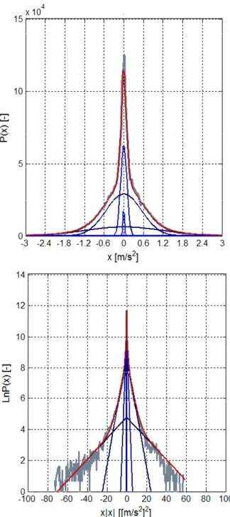
Charles [5] was one among many to recognize that there existed problems relating to the interpretation of vertical vibration data from road vehicles for use to generate laboratory test specifications. He also acknowledged that wheeled vehicle vibrations are “unlikely to be stationary” due to variations in road surface quality and vehicle speed. He also showed that the statistical distribution of vehicle vibrations is more likely to contain larger extrema than that a true Gaussian process as illustrated in Fig. 2.

Figure 2. Illustration of the non-Gaussian nature of vehicle vibrations (after Charles [5]).

Charles [5], who studied a variety of road types, stated: “even for a good classified road, a whole range of surface irregularities may be encountered”. He acknowledged that there exist difficulties associated with distinguishing shocks from vehicle vibrations. Charles [5] suggested that the analysis method for characterising non-stationary vehicle vibrations should include the identification of stationary sections using the “RMS time histogram (sic)” (presumably meaning time history), the examination of vibration severity in terms of RMS and peak amplitude as a function of vehicle speed and verification of the normality of the data by computing the amplitude probability analysis.

Despite the manifest non-stationarity and non Gaussian nature of road vehicle shocks and vibrations, they are not taken into account by most analysis methods in use today. However, more recently, attempts have been made to account for the non Gaussian characteristics of vehicle vibrations by applying a non-linear transformation to a Gaussian function by means of a Hermite polynomial thus

enabling control of the skewness and kurtosis parameters [6,7,8]. The main limitation of this technique is that it fails to recognise that the primary cause of the leptokurtic nature of road vehicles vibrations is the result of the non-stationarity of the process rather than an inherent non-Gaussian character. Consequently, it does not succeed in reproducing the variations in the processes’ amplitude that are considered essential if realistic simulations are to be achieved.

This paper builds on Charles’ proposition that non-stationary random vehicle vibrations consist of Gaussian segments and introduces a method by which measured and numerically-simulated road vehicle vibration data can be decomposed into its constituent Gaussian components.

I. RANDOM GAUSSIAN SEQUENCE DECOMPOSITION

The Probability Distribution Function of a signal composed of a sequence of random Gaussian processes can be expressed as the sum of the individual distribution functions each weighted by, what will here be termed, the Vibration Dose. The Vibration Dose effectively describes the time fraction for which a Gaussian process of a particular standard deviation exists. The decomposition method described here relies on the fact that the distribution function of a sequence of zero-mean Gaussian processes can be described intrinsically as a function of two parameters, namely the vibration dose, Di, and the standard deviation, σi, as follows:

( )

{ }

2 i i i 1

D 1

ln p x ln x x

2πσ 2σ =

⎧ ⎫

⎪ ⎪

= _{⎨ ⎬}−

⎪ ⎪

⎩ ⎭

∑

∑

In this form the function produces a linear relationship between x|x| and ln{p(x)} represented by the slope _{−1/ 2σ}2 and the ordinate intercept ln{D/√2πσ}. This shows that the distribution parameters of a Gaussian process can be determined by fitting a straight line through one half (or side) the distribution estimates to obtain the Vibration Dose and standard deviation as follows:

i i i

i i

1 1

and D 2 exp( C )

2m 2m

σ = = π⋅ −⎛_⎜ ⎞_⎟⋅

⎝ ⎠

(3)

Determine the index, ip, of the first element where ln{p(x)} ≥0 ( p(x) ≥1 )

Set the first boundary bln=ip Initialise the loop counter

n=1

Is ln{p(x)}|minin the range {bln– brn} < 0?

D_n=0 Y

N

Compute the Gaussian estimate standard deviation

and vibration dose. Compute the slope (m) and ordinate intercept (C) of the linearised PDF in the

range { bln– brn} *

Determine the PDF remainder by subtracting the

Gaussian estimate from the PDF of the original record.

Increment the loop counter n=n+1

GOTO *

Compute and plot sum of Gaussian estimates

Tabulate σnand Dnfor all values of n

Y

N

Algorithm commentary

The PDF of the record is computed between limits determined from the absolute minimum and maximum of the entire vibration record. This section of the algorithm deals with determining the optimum region at the ‘tail’ of the distribution function to determine the first Gaussian estimate which, by design, will represent the Gaussian element with the largest standard deviation.

First the element containing the maximum, p(x)maxis identified. Then, elements within the distribution function which contain ‘-inf’ values are detected. These represent elements where p(x) → 0. The very adjacent element toward the centre of the distribution (the mean) is identified and represents the ultimate boundary of the distribution function, bln. The other boundary of the region, brn, is defined as half way between bln and the distribution peak element, ip. This coefficient of ½ was arrived at by experimentation and was found to yield the most consistent and accurate results. The coordinates ln{p(x)} and x|x| within the domain { bln- brn} are used as the first set of values to determine the parameters of the first Gaussian estimate. This is best illustrated in Fig. 4.

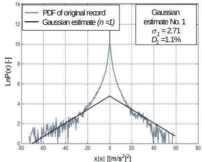
Linear regression by the method of least squares is used to determine the line of best fit through the data and estimates of the slope and ordinate intercept. The Gaussian estimate’s standard deviation (σn) (or RMS for a zero-mean process) and vibration dose (Dn) are computed from estimates of the slope and ordinate intercept. A numerical vector for the Gaussian estimate is generated for the entire range (shown in Fig. 5).

The difference between the original PDF and the Gaussian estimate is computed and used to fit the next Gaussian estimate. The PDF remainder is linearised and any negative value is truncated to zero as a necessity for computing the natural log.

The next range for regression is established by moving the starting point (left boundary, bln) by one and computing the end point (the right boundary, brn) as half way between bln and the PDF peak ip. If the number of elements in the range {bln- brn} is less than 5, it is deemed that there is no longer a sufficient number of points to accurately extract a line of best fit by regression. The programme is terminated and the results displayed as shown in Fig. 6.

Set the other boundary brnto brn=ceiling[ bln+(ip– bln)/2 ]

Set the other boundary brnto brn=ceiling[ bln+(ip– bln)/2 ] Generate Gaussian estimate

Compute the linearised remainder PDF by evaluating x|x| and ln{p(x)}.

Increment the regression domain starting point:

bln= brn-1 + 1

Is (bln– brn) < 5

Figure 3. Random Gaussian Sequence Decomposition algorithm flow chart.

The challenge in developing an automated algorithm to extract a number of Gaussian parameters from a non-Gaussian distribution are related to the data range (or boundary) for each Gaussian element, determining a suitable number of Gaussian elements in the sequence and the effect of fluctuation in the distribution estimates, especially in the high standard deviation, low count region. A description of the algorithm developed in this study is given in Fig. 3 along with illustrations of its operation and the results it generates.

Region for determining the initial Gaussian estimate parameters by

linear regression.

index = bl_n index = br_n

Figure 4. Identification of the region to determine the initial Gaussian estimate parameters by linear regression

PDF of original record Gaussian estimate (n =1)

Gaussian estimate No. 1

σ₁= 2.71

D1=1.1%

Figure 5. First Gaussian estimate along with PDF of original record. Note the relatively small dose that makes

measured vibration records. Although it is acknowledged that the rudimentary nature of the simulation models (only linear elements were used) produces vibration estimates that are not necessarily accurate, the simulation is sufficiently realistic to reproduce the random non-stationarities that occur in reality and are, therefore, deemed adequate to the purpose of this study. The simulation was carried out with a purposed-design program coded in Matlab® and Simulink®. The boundary conditions were accounted for by introducing a vehicle velocity ramp at a constant forward acceleration until the target cruise speed was reached. The vertical vibrations of the quarter-car model were then computed at constant vehicle velocity for the entire pavement profile.

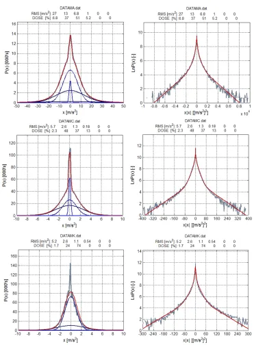
The Random Gaussian Sequence Decomposition method was found to be capable of successfully extracting the Gaussian estimates as well as the corresponding vibration doses for every single test record. Validation was achieved by comparing the sum of these Gaussian estimates against the PDF of the original vibration record. A number of typical results are presented in Fig. 7.

Table I. Summary of measured vibration record parameters.

ID Vehicle type & load Route Type

MA Utility vehicle (1 Tonne capacity). Load: < 5% cap.

S'urban streets MB Prime mover + Semi trailer (Air ride

susp.). Load: 90% cap.

Country roads MC Transport van (700 kg capacity). Load:

60% cap.

Suburban streets MD Transport van (700 kg capacity). Load:

60% cap.

Suburban hwy. ME Transport van (700 kg capacity). Load:

60% cap.

Motorway

MF Prime mover + Semi trailer (leaf spring susp.). Load: < 5% cap.

Country roads MG Tipper truck (16 Tonnes capacity, Air ride

susp.). Load: 25% capacity.

Country roads MH Small flat bet truck (1 Tonne capacity, leaf

spring susp.). Load <5% cap.

Suburban streets MJ Flat bed truck (5 Tonnes capacity, leaf

spring susp.). Load >95% cap.

Country roads MK Sedan car. Load: 1 passenger Suburban

Table II. Summary of routes used for numerically-generated vibration records. ID Route (Victoria, Australia)

SA Murray Valley Highway (Major county road) SB Bendigo – Maryborough road (Major county road) SC Princess Highway (Freeway)

SD Timboon Road, Victoria, Australia (Major county road) SE Road sequence: Timboon Road – Princess Hwy and

Murray Valley Hwy, Victoria, Aust.

PDF of original record Sum of Gaussian estimates

Figure 6. Typical plot of the decomposed Gaussian estimates (blue lines) along with the sum of the Gaussian

estimates (red line) and the PDF of the original record.

II. CONCLUSIONS

attributed to engine vibrations and, although persistent, is insignificant in terms of level and falls below the detection threshold of the algorithm.

REFERENCES

[1] Richards, D.P. “A Review of Analysis and Assessment

Methodologies for Road Transportation Vibration and Shock Data,”

Environmental Engineering, Dec. 1990, pp 23-26. [2] Rouillard, V. & Sek. “Simulation of Non-stationary vehicle

Vibrations,” Proceedings of the Institution of Mechanical Engineers, vol 215, Part D, 2001, pp 1069-1075.

[3] Mil-Std-810E. “Environmental Test Methods and Engineering Guidelines,” US Dept. of Defence, 1989.

[4] Murphy, R.W. “Endurance testing of heavy-duty vehicles,” SAE paper No. SP-506, 1983.

[5] Charles, D. “Derivation of Environment Descriptions and Test Severities from Measured Road Transportation Data,” Journal of the Institute of Environmental Sciences, UK, Feb. 1993, pp 37-42. [6] Steinwolf, A. & Connon, W.H. “Limitations of the Fourier Transform

for Describing Test Course Profiles,” Sound and Vibration Feb. 2005, pp 12-17.

[7] Van Baren, P. “The Missing Knob on your Random Vibration Controller,” Sound and Vibration, Oct. 2005, pp 2-7.

[8] Smallwood, D.O. “Generating Non-Gaussian Vibration for Testing Purposes,” Sound and Vibration, Oct. 2005 pp 18-24.