Complex Stochastic Boolean Systems: Generating and Counting the Binary n-Tuples Intrinsically Less or Greater than u

Complex Stochastic Boolean Systems:

Generating and Counting the Binary

n

-Tuples

Intrinsically Less or Greater than

u

∗

Luis Gonz´alez

†

Abstract—A complex stochastic Boolean system (CSBS) is a system depending on an arbitrary num-ber n of random Boolean variables. The behavior of a CSBS is determined by the ordering between the occurrence probabilitiesPr{u}of the2nassociated bi-naryn-tuplesu= (u₁, . . . , u_n)∈ {0,1}n. In this context, for every fixed binaryn-tuple u, this paper presents two simple algorithms –exclusively based on the vec-tor of positions of the1-bits (0-bits, respectively) inu– for rapidly generating (and counting) all the binary n-tuples v whose occurrence probabilities Pr{v} are always less than or equal to (greater than or equal to, respectively)Pr{u}. Results are illustrated with the intrinsic order graph and they obey to a nice duality property (interchange0s by 1s and “more probable” by “less probable”).

Keywords: complex stochastic Boolean systems, Ham-ming weight, intrinsic order, intrinsic order graph,

(in)comparable binaryn-tuples

1

Introduction

This paper deals with the analysis of complex systems depending on an arbitrary numbernof random Boolean variables, the so-called complex stochastic Boolean sys-tems (CSBSs). That is, then basic variables of the sys-tem are assumed to be stochastic and they only take two possible values: either 0 or 1. Each one of the 2npossible elementary states associated to a CSBS is given by a bi-naryn-tupleu= (u₁, . . . , u_n)∈ {0,1}n of 0s and 1s, and it has its own occurrence probability Pr{(u₁, . . . , u_n)}.

Hence, a CSBS onnvariablesx₁, . . . , x_ncan be modeled by then-dimensional Bernoulli distribution with param-etersp₁, . . . , p_n defined by

Pr{xi= 1}=pi, Pr{xi= 0}= 1−pi,

Throughout this paper we assume that the n Bernoulli variables x_i are mutually statistically independent, so

∗_{Manuscript received July 26, 2009. This work was supported in}

part by the Ministerio de Ciencia e Innovaci´on (Spain) and FEDER through Grant contract: CGL2008-06003-C03-01/CLI.

†_{University of Las Palmas de Gran Canaria, Research}

Insti-tute IUSIANI & Department of Mathematics, 35017 Las Palmas de Gran Canaria, Spain. Email: [email protected]

that the occurrence probability of a given binary string

u= (u₁, . . . , u_n)∈ {0,1}n of lengthncan be easily com-puted as

Pr{u}=

n

i=1

pui

i (1−pi)1−ui, (1.1)

that is, Pr{u}is the product of factorspiifui = 1, 1−pi ifui= 0.

Example 1.1 Let n = 4 and u= (0,1,0,1). Then for

p1 = 0.1, p2 = 0.2, p3 = 0.3, p4 = 0.4, using (1.1), we

have

Pr{(0,1,0,1)}= (1−p₁)p₂(1−p₃)p₄= 0.0504.

The behavior of a CSBS is determined by the ordering between the current values of the 2nassociated binaryn -tuple probabilities Pr{u}. Computing all these 2n prob-abilities –by (1.1)– and ordering them in decreasing or increasing order of their values is only possible in prac-tice for small values of the number nof basic variables. However, for large values ofn, it is necessary to use alter-native procedures for comparing the binary string prob-abilities. For this purpose, in [1] we have established a simple positional criterion that allows one to compare two given binary n-tuple probabilities, Pr{u},Pr{v}, with-out computing them, simply looking at the positions of the 0s and 1s in then-tuplesu, v. We have called it the intrinsic order criterion, because it is independent of the basic probabilitiesp_i and itintrinsically depends on the positions of the 0s and 1s in the binary strings.

Hence, for those pairs (u, v) of binaryn-tuples compara-ble by intrinsic order, the ordering between their occur-rence probabilities is always the same for all sets of basic probabilities {pi}n_i=1. On the contrary, for those pairs (u, v) of binaryn-tuples incomparable by intrinsic order, the ordering between their occurrence probabilities de-pends on the current values of the probabilities{pi}n_i=1.

n-tuple u. In other words, our algorithms –exclusively based on the positions of the 1-bits (0-bits, respectively) ofu– determine the sets of binaryn-tuplesvwhose occur-rence probabilities Pr{v}are always less than or equal to (greater than or equal to, respectively) Pr{u}.

For this purpose, this paper has been organized as fol-lows. In Section 2, we present some previous results on the intrinsic order relation, the intrinsic order graph and other related aspects, enabling non-specialists to follow the paper without difficulty and making the presentation self-contained. Section 3 is devoted to present our new, unpublished results: Two new algorithms and formulas for generating and counting all the binary n-tuples in-trinsically less or greater than u. Finally, in Section 4, we present our conclusions.

2

Background on Intrinsic Order

2.1

Intrinsic Order Relation on

{

0

,

1

}

n

Fist, we must set the following notations. Throughout this paper, the decimal numbering of a binary string u is denoted by the symbol u₍₁₀. We use this symbol, in-stead of the more usual notationu₁₀, to avoid confusions with the 10-th componentu₁₀ of the binary stringu. In the following, we use indistinctly the binary representa-tion or the decimal representarepresenta-tion to denote the elements of{0,1}n, and we represent the conversion between these two numbers systems by the symbol “≡”. Also, the Ham-ming weight of a binary n-tuple u (i.e., the number of 1-bits inu) will be denoted, as usual bywH(u), i.e.,

(u₁, . . . , un)≡u₍₁₀ =

n

i=1

2n−iui, wH(u) =

n

i=1

ui,

e.g., forn= 5 we have

(1,0,1,1,1)≡20+21+22+24= 23, wH(1,0,1,1,1) = 4.

According to (1.1), the ordering between two given binary string probabilities Pr (u) and Pr (v) depends, in general, on the parameterspi of the Bernoulli distribution, as the following simple example shows.

Example 2.1 Letn= 3, u= (0,1,1) andv= (1,0,0). Using (1.1) we have

Forp₁= 0.1, p₂= 0.2, p₃= 0.3:

Pr{(0,1,1)}= 0.054<Pr{(1,0,0)}= 0.056,

forp₁= 0.2, p₂= 0.3, p₃= 0.4:

Pr{(0,1,1)}= 0.096>Pr{(1,0,0)}= 0.084.

As mentioned in Section 1, to overcome the exponential complexity inherent to the task of computing and sorting

the 2n binary string probabilities (associated to a CSBS withnBoolean variables), we have introduced the follow-ing intrinsic order criterion [1], denoted from now on by the acronym IOC (see [5] for the proof).

Theorem 2.1 (The intrinsic order theorem) Let

n ≥ 1. Let x₁, . . . , x_n be n mutually independent Bernoulli variables whose parameters p_i = Pr{x_i= 1} satisfy

0< p₁≤p₂≤ · · · ≤p_n≤0.5. (2.1)

Then the probability of the n-tuple v = (v₁, . . . , vn) ∈

{0,1}n is intrinsically less than or equal to the probability of the n-tupleu= (u₁, . . . , un)∈ {0,1}n (that is, for all set{p_i}n_i=1 satisfying(2.1))if and only if the matrix

Mu v :=

u1 . . . un

v1 . . . vn

either has no1₀columns, or for each1₀column inM_vu there exists(at least)one corresponding preceding0₁ col-umn(IOC).

Remark 2.1 In the following, we assume that the pa-rametersp_ialways satisfy condition (2.1). Note that this hypothesis is not restrictive for practical applications be-cause, if for somei:p_i>1₂, then we only need to consider the variablex_i= 1−x_i, instead ofx_i. Next, we order the

nBernoulli variables by increasing order of their proba-bilities.

Remark 2.2The0₁column preceding to each 1₀ col-umn is not required to be necessarily placed at the imme-diately previous position, but just at previous position.

Remark 2.3The termcorresponding,used in Theorem 2.1, has the following meaning: For each two1₀columns in matrix M_vu, there must exist (at least) two different

₀ 1

columns preceding to each other. In other words: For each1₀column in matrixM_vu, the number of preceding

₀ 1

columns must be strictly greater than the number of preceding1₀columns.

The matrix condition IOC, stated by Theorem 2.1, is called the intrinsic order criterion, because it is inde-pendent of the basic probabilitiesp_i and it intrinsically depends on the relative positions of the 0s and 1s in the binaryn-tuplesu, v. Theorem 2.1 naturally leads to the following partial order relation on the set{0,1}n [1]. The so-called intrinsic order will be denoted by “”, and we shall writevu(uv) to indicate thatv (u) is intrin-sically less (greater) than or equal tou(v).

Definition 2.1 For all u, v∈ {0,1}n

vu iff Pr{v} ≤Pr{u} for all set {pi}n_i=1 s.t. (2.1)

From now on, the partially ordered set (poset, for short) ({0,1}n,) will be denoted byI_n.

Example 2.2 For n = 3: 3 ≡ (0,1,1) 4 ≡ (1,0,0), 4≡(1,0,0)3≡(0,1,1) because the matrices

1 0 0 0 1 1

and

0 1 1 1 0 0

do not satisfy IOC (Remark 2.3). Thus, (0,1,1) and (1,0,0) are incomparable by intrinsic order, i.e., the ordering between Pr{(0,1,1)}and Pr{(1,0,0)}depends on the parameters{p_i}3_i=1, as Example 2.1 has shown.

Example 2.3 For n = 5: 24 ≡ (1,1,0,0,0) 5 ≡ (0,0,1,0,1) because matrix

0 0 1 0 1 1 1 0 0 0

satisfies IOC (Remark 2.2). Thus, for all{pi}5_i=1 s.t. (2.1)

Pr{(1,1,0,0,0)} ≤Pr{(0,0,1,0,1)}.

Example 2.4 For alln≥1, the binary n-tuples

0,. . .,n 0 ≡0 and

1,. . .,n 1 ≡2n−1

are the maximum and minimum elements, respectively, in the posetI_n. Indeed, both matrices

0 . . . 0

u1 . . . un

and

u1 . . . un

1 . . . 1

satisfy the intrinsic order criterion, since they have no1₀ columns!.

Thus, for allu∈ {0,1}n and for all{pi}n_i=1 s.t. (2.1)

Pr

1,. . .,n 1 ≤Pr{(u₁, . . . , un)} ≤Pr

0,. . .,n 0 .

2.2

The Intrinsic Order Graph

To finish this Section, we present the graphical represen-tation of the posetIn. The usual representation of a poset is its Hasse diagram (see, e.g., [6] for more details about posets and Hasse diagrams). This is a directed graph (di-graph, for short) whose vertices are the binary n-tuples of 0s and 1s, and whose edges go downward fromuto v wheneverucoversv (denoted byu v), that is, whenever

uis intrinsically greater than v with no other elements between them, i.e.

uv iff u vand there is now∈ {0,1}n s.t.u w v.

The Hasse diagram of the poset I_n will be also called the intrinsic order graph for n variables. For all n ≥

2, in [3] we have developed an algorithm for iteratively building up the digraph of I_n from the digraph of I₁. Basically,I_nis obtained by adding toI_n−1its isomorphic copy 2n−1+I_n−1: A nice fractal property ofI_n!

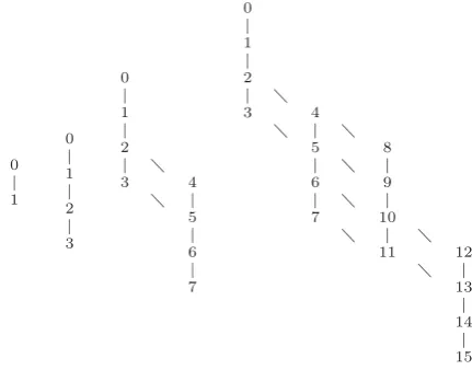
In Fig. 1, the intrinsic order graph for n = 1,2,3,4 is shown, using the decimal numbering instead of the bi-nary representation of their 2n nodes, for a more com-fortable and simpler notation. Each pair (u, v) of vertices connected in the digraph ofIn either by one edge or by a longer descending path (consisting of more than one edge) from u to v, means that uis intrinsically greater thanv, i.e., u v. On the contrary, each pair (u, v) of non-connected vertices in the digraph ofI_n either by one edge or by a longer descending path, means thatuandv are incomparable by intrinsic order, i.e.,uvandvu.

0

|

1 0

|

1

|

2

|

3 0

|

1

|

2

|

3 4

|

5

|

6

|

7 0

|

1

|

2

|

3 4

|

5 8

| |

6 9

| |

7 10

|

11 12

|

13

|

14

|

[image:3.595.309.525.304.473.2]

15

Fig. 1. The intrinsic order graph forn= 1,2,3,4.

2.3

The Sets

C

u

and

C

u

Many different properties of the intrinsic order relation can be derived from its simple matrix description IOC (see, e.g., [1, 2, 3]). For the purpose of this paper, we must recall here the following necessary (but not suffi-cient) condition for intrinsic order; see [2] for the proof.

Corollary 2.1 For all u, v∈ {0,1}n

uv ⇒ wH(u)≤wH(v).

Definition 2.2 For every binary n-tuple u ∈ {0,1}n,

Cu _(C

u, respectively) is the set of all binary n-tuples v whose occurrence probabilities Pr{v} are always less (greater, respectively) than or equal toPr{u}, i.e., those

n-tuplesv intrinsically less(greater, respectively)than or equal tou, i.e.,

Cu_{={v∈ {0,1}}n _{|Pr{u} ≥Pr{v},∀ {p}

i}ni=1 s.t. (2.1)},

In other words, according to Definition 2.1,

Cu_{={v∈ {0,1}}n _{|u v}, (2.2)} Cu={v∈ {0,1}n |uv}. (2.3)

For instance, due to Example 2.4, we have, for alln≥1,

C

„ 0,_...,n₀«

={0,1}n=C„

1,_...,n₁«,

as Fig. 1 shows, forn= 1,2,3,4.

The setsCu and Cu are closely related via complemen-taryn-tuples, as described with precision by the following definition and theorem [4].

Definition 2.3 The complementary n-tuple of a binary

n-tupleu ∈ {0,1}n is obtained by changing its 0s by 1s and its1s by0s

uc_{= (u}

1, . . . , un)c = (1−u1, . . . ,1−un).

The complementary set of a setS ⊆ {0,1}n of binaryn -tuples is the set of the complementaryn-tuples of all the

n-tuples ofS

Sc_={uc _|u∈S}.

Theorem 2.2 For alln≥1 and for allu∈ {0,1}n

Cu=

Cucc

, Cu_{= [Cuc]}c_{. (2.4)}

3

The Algorithms

This Section is devoted to present our new results. First, we need to set the following nomenclature and notation.

Definition 3.1 Letn≥1 and letu∈ {0,1}nwith Ham-ming weightw_H(u) =m. Then

(i) The vector of positions of 1s of u is the vector of positions of its m 1-bits, displayed in increasing order from the left-most position to the right-most position, and it will be denoted by

u=i1₁, . . . , i1_m1_n, 1≤i1₁<· · ·< i1_m≤n, 0< m≤n.

(ii)The vector of positions of0s of uis the vector of po-sitions of its(n−m) 0-bits, displayed in increasing order from the left-most position to the right-most position, and it will be denoted by

u=i0₁, . . . , i0_n−m0_n, 1≤i0₁<· · ·< i0_n−m≤n, 0≤m < n.

Example 3.1 For n = 6 and u = 27≡ (0,1,1,0,1,1), we havem=w_H(u) = 4,n−m= 2, and

u=i1₁, i1₂, i₃1, i1₄1₆= [2,3,5,6]1₆, u=i0₁, i0₂0₆= [1,4]0₆.

In [4], the authors present an algorithm for obtaining the set Cu, for each given binary n-tuple u. Basically, this algorithm determinesCu by expressing the set difference

{0,1}n−Cu as a set union of certain half-closed inter-vals of natural numbers (decimal representation of binary strings). The next two theorems present new, more ef-ficient algorithms for rapidly determining Cu and Cu, using the binary representation of their elements. More-over, our new algorithms allow us not only to generate, but also to count the number of elements ofCu andCu.

Theorem 3.1 (The algorithm forCu) Let u ∈

{0,1}n, u = 0, with weight w_H(u) = m (0< m≤n). Let u =i1₁, . . . , i1_m1_n be the vector of positions of 1s of

u. ThenCu is the set of binary n-tuples v generated by the following algorithm:

(i)Step 1(Generation of the sequencesj1₁, . . . , j1_m) :

Forj1₁= 1 toi1₁ Do:

Forj₂1=j₁1+ 1toi1₂ Do:

· · · ·

Forj_m1 =j_m−1 ₁+ 1 toi1_m Do:

Writej₁1, j₂1, . . . , j_m1

EndDo

· · · ·

EndDo

EndDo

(ii)Step 2(Generation of then-tuplesv∈Cu) :

For every sequencej1₁, . . . , j_m1generated by Step 1, de-finev= (v₁, . . . , vn)as follows

vi=

⎧ ⎨ ⎩

1 if i∈j₁1, . . . , j_m1,

0 if i /∈j₁1, . . . , j_m1, i < j1_m, 0,1 if i /∈j₁1, . . . , j_m1, i > j1_m.

(3.1)

Moreover, the cardinality of the set Cu is given by the multiple sum

|Cu_|= i1

1

j1 1=1

i1 2

j1 2=j11+1

· · ·

i1

m

j1

m=jm1−1+1

2n−j1m. _(3.2)

Proof. Note that, according to (2.2) and Corollary 2.1, we have

v∈Cu_⇔uv⇒m=w

H(u)≤wH(v),

First, we generate all binary n-tuples v ∈ Cu with weight m. Let v ∈ {0,1}n with w_H(v) = m and let

v=j₁1, . . . , j1_m1_n be the vector of positions of 1-bits ofv. Using (2.2) and IOC (Theorem 2.1), we have thatv∈Cu if and only if

u=i1₁, . . . , i1_m1_nj₁1, . . . , j_m11_n=v,

if and only if v contains at least one 1-bit among the positions 1 andi1₁, at least two 1-bits among the positions 1 andi1₂,. . ., at least (m−1) 1-bits among the positions 1 andi1_m−1, exactlym 1-bits among the positions 1 and

i1

m, and (ifi1m< n)v has no 1-bits among the positions i1

m+ 1 andn. That is,v∈Cu,wH(v) =mif and only if

1≤j1₁≤i₁1, j₁1+ 1≤j₂1≤i1₂, . . . , j_m−1 ₁+ 1≤j_m1 ≤i1_m, (3.3) and these are exactly the sequences j₁1, . . . , j_m1 gen-erated by Step 1. Hence, the binary n-tuples v ∈ Cu with the same weight m as u are exactly the n-tuples

v = j₁1, . . . , j_m11_n, that is, those binary n-tuples v de-fined by Step 2, when we choosev_i = 0 for alli > j_m1. In addition, by the way we derive that the number of those

n-tuples is exactly

|{v∈Cu _|w

H(v) =m}|= i1

1

j1 1=1

i1 2

j1 2=j11+1

· · ·

i1

m

j1

m=j1m−1+1

1.

Second, we generate all binaryn-tuplesv∈Cu (with all possible weightsw_H(v)≥m). Once we have character-ized all n-tuples v ∈ Cu with wH(v) = m = wH(u), the question is quite simple. Indeed, let u v with

wH(v) = t ≥ m. Let j1₁, . . . , j_m1 be the sequence of positions of the m left-most 1-bits of v. Then, on one hand, according to IOC, this sequence must necessarily satisfy (3.3) (i.e., it must be one of the sequences gen-erated by Step 1). On the other hand, note that the substitution of 0s by 1s in anyn-tuplev such thatuv does not avoid the IOC condition, because this substitu-tion changes the0₀and1₀columns of matrixM_vu into

₀ 1

and 1₁ columns, respectively. Hence, to obtain all the binary strings of the setCu, it is enough to assign, in all possible ways, both values, either 0 or 1, to any of the n−j1_m (if j_m1 < n) null right-most components

vj1

m+1,· · · , vn of all the binary strings v=

j1

1, . . . , jm1

₁

n

with eight m, generated by (3.3). In other words, we definev as described by (3.1).

Finally, since there are exactly 2n−jm1 different ways of assigning the values v_i = 0,1 for all j_m1 < i ≤ n, and since by this procedure we generate all elements of Cu without repetitions, then the cardinality of Cu is given

by (3.2).

Theorem 3.2 (The algorithm forC_u) Letu∈ {0,1}n,

u= 2n−1, with weight w_H(u) =m (0≤m < n). Let

u=i0₁, . . . , i0_n−m0_n be the vector of positions of 0s ofu. ThenCu is the set of binaryn-tuples v generated by the following algorithm:

(i)Step 1(Generation of the sequencesj₁0, . . . , j_n−m0 ) :

Forj0₁= 1 toi0₁ Do:

Forj₂0=j₁0+ 1toi0₂ Do:

· · · ·

Forj_n−m0 =j_n−m−0 ₁+ 1toi0_n−m Do:

Writej₁0, j₂0, . . . , j_n−m0

EndDo

· · · ·

EndDo

EndDo

(ii)Step 2(Generation of then-tuplesv∈Cu) :

For every sequence j₁0, . . . , j_n−m0 generated by Step 1, definev= (v₁, . . . , vn)as follows

vi=

⎧ ⎨ ⎩

0 if i∈j₁0, . . . , j_n−m0 ,

1 if i /∈j₁0, . . . , j_n−m0 , i < j0_n−m, 0,1 if i /∈j₁0, . . . , j_n−m0 , i > j0_n−m.

(3.4)

Moreover, the cardinality of the set C_u is given by the multiple sum

|Cu|=

i0 1

j0 1=1

i0 2

j0 2=j10+1

· · ·

i0

m

j0

n−m=jn0−m−1+1

2n−jn0−m. _(3.5)

Proof. For proving this theorem, it is enough to use Theorems 2.2 and 3.1. Indeed, due to the left-hand set equality of Theorem 2.2, obtaining the setCu is equiva-lent to obtaining the setCucc.

First, we obtain the set Cuc using Theorem 3.1. Since the (n−m) 1-bits ofuc are placed at the same positions as the (n−m) 0-bits of u (i.e., i0₁, . . . , i0_n−m), then the sequences foruc, generated by Step 1 in Theorem 3.1, are exactly the sequencesj₁0, . . . , j0_n−mforu, generated by Step 1 in Theorem 3.2. Thus, all binaryn-tuplesv∈Cuc can be obtained by applying Step 2 in Theorem 3.1 to each one of the sequencesj₁0, . . . , j_n−m0 , generated by Step 1 in Theorem 3.2.

Second, once we have obtained the set Cuc, for obtain-ing the setCucc, we only need to take the complemen-tary n-tuples of alln-tuples v ∈ Cuc. That is, we only need to change the 0s by 1s and the 1s by 0s in all n -tuples v ∈ Cuc, obtained from (3.1) for the sequences

j0

1, . . . , jn−m0

Finally, (3.5) follows immediately using the fact that

|Cu|=Cucc=Cucand (3.2).

Remark 3.1 Note the strong duality relation between Theorems 3.1 and 3.2. The statement of each theorem is exactly the statement of the other one after interchanging 1s and 0s,Cu andCu. Indeed, due to Theorem 2.2, one can determine the setCu(Cu, respectively) by determin-ing the set [Cuc]c (Cucc, respectively) using Theorem

3.2 (Theorem 3.1, respectively).

Remark 3.2Letu∈ {0,1}n be a fixed binaryn-tuple. On one hand,v∈ {0,1}nis comparable by intrinsic order withuif either uv or uv, i.e., if either v ∈Cu or

v ∈ Cu, respectively (see Definition 2.2). On the other

hand, due to the reflexivity and antisymmetry properties of the intrinsic order relation, we have Cu∩C_u ={u}. Hence, the number of binaryn-tuplesvincomparable by intrinsic order withuis given by

|{v∈ {0,1}n |u v, u⊀ v}|= 2n+ 1− |Cu| − |Cu|. (3.6)

The following example illustrates Theorems 3.1 and 3.2.

Example 3.2 Letn= 4 andu= 6≡(0,1,1,0). Then, we havem=w_H(u) = 2,n−m= 2, and

u=i1₁, i₂11₄= [2,3]1₄, u=i0₁, i0₂0₄= [1,4]0₄.

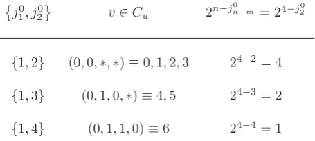
[image:6.595.307.535.156.258.2]

Using Theorems 3.1 and 3.2 we can generate all the 4-tuplesv ∈ Cu and all the 4-tuples v ∈Cu, respectively. Results are depicted in Tables I and II, respectively. The first column of Tables I and II, show the auxiliary se-quences generated by Step 1 in Theorems 3.1 and 3.2, respectively. The second column of Tables I and II, show all the binary 4-tuplesv ∈Cu andv ∈C_u generated by Step 2 in Theorems 3.1 and 3.2, respectively. The sym-bol “∗” means that we must choose both binary digits: 0 and 1, as described by the last line of (3.1) and (3.4). According to (3.2) and (3.5), the sums of all quantities in the third column of Tables I and II, give the number of elements ofCu andC_u, respectively, using just the first columns and then with no need to obtain these elements by the second columns.

Table I. The setC(0,1,1,0)and its cardinality.

j1 1, j21

v∈Cu ₂n−j1

m _{= 2}4−j21

{1,2} (1,1,∗,∗)≡12,13,14,15 24−2= 4

{1,3} (1,0,1,∗)≡10,11 24−3= 2

{2,3} (0,1,1,∗)≡6,7 24−3= 2

So, Cu = {6,7,10,11,12,13,14,15} and |Cu| = 8 (see the digraph ofI₄, the right-most one in Fig. 1).

Table II. The setC_(0,1,1,0) and its cardinality.

j0 1, j20

v∈Cu 2n−j0n−m_{= 2}4−j02

{1,2} (0,0,∗,∗)≡0,1,2,3 24−2= 4

{1,3} (0,1,0,∗)≡4,5 24−3= 2

{1,4} (0,1,1,0)≡6 24−4= 1

So,Cu={0,1,2,3,4,5,6} and|Cu|= 7 (see the digraph ofI₄, the right-most one in Fig. 1).

Finally, the binary n-tuples v incomparable by intrinsic order withu= (0,1,1,0) are{0,1}n−(Cu∪C_u) ={8,9} (see the digraph ofI₄, the right-most one in Fig. 1). So, they are exactly 2n+ 1− |Cu| − |C_u|= 16 + 1−8−7 = 2 binary strings, in accordance with (3.6).

4

Conclusions

The two dual algorithms presented in this paper for rapidly generating and counting the setsCu and Cu are exclusively based on the positions of the 1-bits or 0-bits, respectively, of u, and they are easily implementable. Hence, results can be applied to any CSBS with an arbi-trarily large numbernof independent Boolean variables.

References

[1] Gonz´alez, L., “A New Method for Ordering Binary States Probabilities in Reliability and Risk Analy-sis,” Lect Notes Comp Sc, V2329, N1, pp. 137-146, 2002.

[2] Gonz´alez, L., “N-tuples of 0s and 1s: Necessary and Sufficient Conditions for Intrinsic Order,”Lect Notes Comp Sc, V2667, N1, pp. 937-946, 2003.

[3] Gonz´alez, L., “A Picture for Complex Stochastic Boolean Systems: The Intrinsic Order Graph,”Lect Notes Comput Sc, V3993, N3, pp. 305-312, 2006.

[4] Gonz´alez, L., “Algorithm comparing binary string probabilities in complex stochastic Boolean systems using intrinsic order graph,”Adv Complex Syst, V10, N1, pp. 111-143, 2007.

[5] Gonz´alez, L., Garc´ıa, D., Galv´an, B., “An Intrinsic Order Criterion to Evaluate Large, Complex Fault Trees,”IEEE Trans on Reliability, V53, N3, pp. 297-305, 2004.