On Vector Fitting Methods in Signal/Power Integrity Applications

On Vector Fitting Methods in Signal/Power

Integrity Applications

Chi-Un Lei

†

, Yuanzhe Wang, Quan Chen and Ngai Wong

Abstract—Vector Fitting (VF) has been applied to reformu-late traditional system identification techniques by introducing a partial-fraction basis to avoid ill-conditioned calculation in broadband system identifications. Because of the reliable and versatility of VF, many extensions and applications have been proposed, for example, the macromodeling of linear structures in signal/power integrity analyses. In this paper, we discuss the macromodeling framework and some main features in VF in terms of data, algorithms and models. Finally, an alternative P-norm approximation criterion is proposed to enhance the macromodeling process.

Index Terms—Signal/Power Integrity, Vector Fitting, Macro-modeling, Tutorial, Approximation

I. INTRODUCTION

Vector Fitting (VF) [1] is a numerical technique for sam-pled response-matching system identification (macromodel-ing), which involves iterative linear least-squares solves with a partial fraction basis. As opposed to other system identification techniques for broadband (from DC to GHz) system identi-fication, VF avoids ill-conditioned calculation, and therefore works in a more robust and efficient manner. Furthermore, its theoretically-simple and versatile framework can easily incooperate various constraints by introducing a variety of extensions for other areas. VF has also been used in modeling of different electrical systems [1], [2] and extended to differ-ent areas, for example, filter design [3]–[5], power network analysis [2], [6] and electromagnetic (EM) simulation [7].

The idea of VF was firstly introduced for transmission line transient modeling in [8]. The underlying idea of VF is to replace the approximated (or initialized) poles with an improved set of poles through implicit weighting (the pole relocation technique), which thereby improves the approxima-tion iteratively. VF approximates an underlying system to a new system using partial fraction basis with real or complex conjugate poles. A number of generalizations and extensions have been proposed for better VF performance and integration with various identification requirements [9]–[24]. VF has been thoroughly discussed in [25], [26]. Its basic implementation is available from [27], whereas its variants have been widely used in industrial electronic design workflows for signal integrity issues [28]–[30].

This paper acts as a tutorial on VF. We first give a brief introduction to the signal/power integrity issues (Section II)

†_{Corresponding Author.}

[image:1.612.320.541.176.274.2]

C-U. Lei, Y. Wang, Q. Chen and N. Wong are with the Department of Electrical and Electronic Engineering, The University of Hong Kong, Pokfulam Road, Hong Kong. Phone: ++852 +2859 2698 Fax: ++852 +2559 8738 Email:{culei, yzwang, quanchen, nwong}@eee.hku.hk

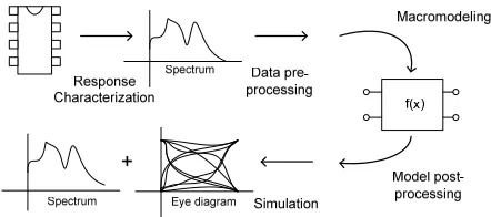
Fig. 1. Common macromodeling flow in signal integrity analyses.

and basic formulation of VF (Section III). Then we discuss the applications of VF in system identification (Sections IV, V and VI). Finally an alternative P-norm approximation cri-terion in VF is proposed for approximation enhancement (Section VII), which is verified through numerical examples (Section VIII).

II. MACROMODELING: SYSTEMIDENTIFICATION PROBLEM INSIGNAL/POWERINTEGRITY

With the increasing operational frequency and decreasing size of integrated circuits (ICs), high-frequency effects, such as signal delay and crosstalk, have become dominant factors lim-iting system performance in IC design. Accurate and efficient simulation is required to capture the high-frequency behavior of systems, so as to ensure consistent transmissions and reli-able ground (and power) distributions in high-speed electronic systems [2], [31]. A common simulation flow is shown in Fig. 1. The sampled structure responses can be obtained by ex-citing one input port at a time and computing or measuring the responses at the output ports (Response Characterization). By approximating the sampled frequency-dependent or time-dependent system response data, a macromodel is generated to replace the original large-order system by a smaller-order one with similar input-output relationship (Macromodeling). The macromodel is used to generate spectra and waveforms for signal integrity analysis or coupled with other circuit model blocks (e.g., logic devices) for global simulation (Simulation). Peripheral pre-processing and post-processing techniques are used to rectify the macromodel characteristics and enhance the simulation performance.

Generally, for a single-port (one input port and one out-put port) system, macromodeling techniques intend to fit a linear-time invariant (LTI) system to the desired continuous-time frequency-sampled response H(s) at a set of calcu-lated/sampled points at the input and output ports. The model

is usually a state-space system or a rational transfer function with a set of basis {φn}

H(s)≈N(s)

D(s) =

N

X

n=1

bnφn(s)

,_XN

n=1

ebnφn(s), (1)

where ebn, bn ∈ ℜ and N is the macromodel order. The algorithm is usually required to fit hundreds of sampled data points for each port. Therefore, the linear-structure macro-modeling can be classified as a large-scale broadband system identification problem. There are many strict constraints in this macromodeling procedure, such as accurate and physically-consistent response approximation, low computation complex-ity, and numerically-robust computation in the broadband, massive-ports (massive-coupled) and large-order system mod-eling cases.

In the L2 sense, the optimal model of a system can be

obtained through minimizing the following objective function

min N(s)

D(s) −H(s)

2 . (2)

However, this is a numerically-sensitive non-linear problem with no prior information about the exact pole and zero loca-tions of the system under identification. The response is usu-ally approximated using Prony’s method [32] for a coarse so-lution or other identification frameworks, such as continuous-time domain Sanathanan-Koerner (SK) iteration [33] or equiv-alent discrete-time domain counterpart [34], for a finer so-lution. The objective function of the SK iteration in the tth iteration is min

N(t)_(s) D(t−1)_(s)−

D(t)_(s) D(t−1)_(s)H(s)

2 . (3)

By arranging the weighting function σ(t)_{(s) :=} D(t)_(s)D(t−1)_{(s), the model parameters can be determined}

using a least-squares solving

N(t)_(s) D(t)_(s)

D(t)_(s) D(t−1)_(s)

| {z }

(σH)(t)_(s)

− D

(t)_(s)

D(t−1)_(s)

| {z }

σ(t)_(s)

H(s)≈0

. (4)

If a monomial power series basis function is used in (4) for broadband macromodeling, i.e., φn(s) =sn, the traditional SK iteration approach will suffer from an ill-conditioned Vandermonde matrix calculation [9]. Therefore, Vector Fitting (VF) is proposed as a robust and simple broadband macromod-eling technique, which has been widely applied in practice. In this paper, the discussion of VF is divided into three sections:

1) Data section (H(s)): Input data choices (Section IV-A), pre-processing of data (Section IV-B) and model (Sec-tion IV-C);

2) Algorithms section (H(s)→N(s)/D(s)): Identifica-tion criterion and framework (SecIdentifica-tion V-A) and numer-ical implementation (Section V-B);

3) Models section (N(s)/D(s)): Post-processing for model physical consistency (Section VI-A) and simu-lation (Section VI-B).

III. FORMULATION OFVECTORFITTING(VF)

In VF, given a set of poles{αn}, (1) is approximated using a summation of partial fraction basis and a unity basis with their model parameters{cn} andd,

H(s)≈ N(s)

D(s) =

N

X

n=1 cn

s+αn

!

+d. (5)

By including the weighting function σ(s), (5) is linearized into an iterative separable denominator calculation, namely, for thetth iteration,

N

X

n=1

c(t)n

s+α(t)n

! +d(t)

| {z }

σH(t)_(s)

≈ _N

X

n=1

γ(t)n

s+α(t)n

! + 1

!

| {z }

σ(t)_(s)

H(s) , (6)

which falls into the framework of SK iteration (4) [9], [10]. In numerical implementation, provided all poles are real and

Ns frequency-sampled data points are given, an expression from (6) is formed for each frequency-sampled point si,i=

1,2, . . . , Ns,

Aix=bi, (7)

where bi = H(si), x =

h

c₁(t) · · · c_N(t) d(t) _γ(t)

1 · · · γ (t)

N

i

, and

Ai =

h ₁

s+α(t)₁ · · ·

1

s+α(t)n

1 −H(si)

s+α(t)₁ · · ·

−H(si)

s+α(t)n

i

.

xare solved through stacking the row (7) at the Ns sampled points to form an overdetermined linear equations problem,

AT

1 AT2 · · · ATNs

T

x= b1 b2 · · · bNs

T

,

(8)

where it can be solved through normal equations or a QR decomposition. The zeros ofσ(t)_{(s)(i.e., the new set of poles}

n

αn(t+1)

o

) can be calculated as the eigenvalues of the matrix

Ψ =      

α₁(t) α(₂t)

. ..

α(_Nt)

     −      1 1 .. . 1           

γ₁(t) γ₂(t)

.. .

γ_N(t)

      T . (9)

If the poles are unstable (i.e.,ℜnα(nt+1)

o

>0), the poles are flipped against the imaginary axis to the open left half plane for pole stabilization

α(nt+1):=−α

(t+1)

n . (10)

This is equivalent to cascading an allpass filterA(s)to alter the phase response

A(s) = s+α

s−α. (11)

The computation is repeated until convergence is achieved, say, σ(s) ≈ 1 and _DN(t)(t)(_(ss₎)−H(s)

≈ 0, at the NTth iterations. Eq. (6) is then reduced to

N

X

n=1

c(NT)

n

s+α(NT)

n

+d(NT)

≈H(s), (12)

and the residues nc(NT)

n

o

andd{NT} _{can be calculated}

simi-larly as in (8). In summary, VF replaces the monomial power series basis by a partial fraction basis, which significantly improves the numerical condition in calculation of (8). The detailed VF formulation is shown in [1], [9], [10]. Pseudocodes are given to summarize the framework of VF:

Algorithm 1 Pseudocodes of Vector Fitting (VF)

1: FindH(z), and assign

n

α(0)n

o

; 2: repeat

3: Calculatenγn(t)

o

by solving (8) withnα(nt)

o

;

4: Calculate nα(nt+1)

o

by solving (9) and stabilize the unstable poles through (10);

5: untilnαn(t)

o

converges after NT iterations

6: Calculate nc(NT)

n

o

and d(NT) _{through (12) with}

n

α(NT)

n

o

;

IV. DATA

Data describe the system response, and are obtained from measurements (e.g., vector network analyzer (VNA)) or EM simulators (e.g., Nexxim [30]). Since data content can affect the properties and quality of the macromodel, different con-siderations and techniques have been proposed to ensure the input data are maximally informative for identification.

A. Input data choices

Continuous-time frequency-sampled dataH(s)are used for macromodeling in VF [1], as the frequency-sampled responses capture the high-frequency behaviors of the system. Exam-ples of frequency-sampled data are scattering parameters (S -parameters) for RF objects and admittance parameters (Y -parameters) for interconnects. Alternative data choices, such as frequency response derivative H′_{(s) [15], phase response}

∠H(s) [16] and magnitude response |H(s)| [17], are used for different identification purposes. In practices, frequency-domain macromodeling involves complicated measurements. Truncated time-sampled data (input and output responseX[n]

and Y [n]) are often used, therefore (discrete) time-domain VF have been proposed [13], [14]. Approximation using combination of several classes of data (hybrid-domain ap-proximation) provides extra system information for a more accurate approximation. It has been applied to digital IIR filter approximation [4] and works well in macromodeling process.

B. Pre-processing of data

The system response should correctly describe the system. However, some problems, such as data burst, defects, missing and noise-disturbance, may happen during data collection. Some information may get lost and difficulties and failures in approximation may arise. Therefore, data pre-processing is required to ensure the data are meaningful (e.g., passive and

causal, as explained in Section VI-A) to generate a correct macromodel. For example, causality and passivity verifica-tion of input data and delay extracverifica-tion using (generalized) Hilbert transform [35] are developed. Furthermore, causality-constrained data interpolation is developed to generate con-sistent DC and low-frequency data, which is necessary for simulation but usually not provided in the frequency-sampled data [35].

In addition, a large data set or broadband responses usu-ally have a large variance and may result in ill-conditioned calculation. Pre-filtering techniques, in this scenario, can be used to change the distribution of noise and bias, so as to give a better fitting of important frequency range and a numerically favorable calculation with a small computational cost. An appropriate adaptive or deterministic data selection process and response weighting can also be applied for a better approximation.

C. Pre-processing of model

A priori configuration of macromodels should be chosen based on the knowledge of the algorithms (SK iteration) and data for a convenient approximation. For example, an

a priorimodel order selection helps generate a minimum size macromodel for efficient simulations with accuracy control. The model order can be selected by applying experimental observation of the frequency response in frequency-sampled data [18], or the Hankel Singular Value (HSV) in (discrete) time-sampled data [14].

V. ALGORITHMS

Given a set of input data, an algorithm is used to determine the model parameters. A good algorithm should have an ap-propriate identification criterion and should be easy and robust for numerical implementation. We first discuss the algebraical minimization criteria, then the numerical implementation for a numerically favorable model parameters calculation.

A. Identification criterion and framework

The selection of the approximation criteria is important for model approximation. The model should be reliable, obtained within a reasonable computation time, and should admit an exact description of the true system. SK iteration with anL2

-norm prediction error is usually used since it is applicable to different response models. Other criterion extensions are also developed recently for specific applications.

Massive-port macromodeling: VF handles multi-port macromodeling by stacking the system equation matrices of responses of all ports into a single column of over-determined equation for solutions. However, numerical difficulties ex-ist in modeling the systems with a large number of ports (e.g., package parasitic networks and electromagnetic-aware circuits). To model a system with an arbitrary number of ports, a reformation of the VF framework is proposed to approximate the eigenpairs rather than the matrix elements [20]. It gives a more accurate approximation for systems with a large ratio between the largest and smallest eigenvalues.

Parametric macromodeling: Variabilities in geometry and material properties are generated during the manufacturing process, and become a critical factor in nano-scale high-frequency circuit simulation and design. In order to accurately predict the behavior and reduce the computation time of repeated simulations, a parametric macromodel is used to describe the variational structures

H(s, g)≈

PNs

n=0

PP

p=1bnpϕp(g)

φn(s)

PNs

n=0

PP

p=1ebnpϕp(g)

φn(s)

, (13)

where φn(s) is the frequency-dependent basis and ϕp(g) is the variability-dependent basis with a single variational parameter g and P samples in the variability domain. The variational structures can be described by a macromodel with a polynomial basis or rational function basis [23], [24], [26].

B. Numerical Implementation

Due to the nature of iterative calculation, its implemen-tation is usually numerically sensitive. Although VF solves the ill-conditioned calculation by a partial-fraction basis, other problems, such as inappropriate initial guess and noise-contaminated responses, damage the algorithm convergence. Some improvements have been proposed to alleviate these problems.

Initial poles and applied basis: The algorithm gives a set of model parameters (bn and˜bn in (1)) according to the given set of basis (φ(s)), the sampled data and the initial poles. The selected basis affects the conditioning of the system equation matrix in (8) and the accuracy of the solution.

One approach to address this problem is to select an appropriate set of initial poles. The initial poles can be obtained by a simple calculation (e.g., Prony method [32]), or intuitively assigned as a set of weakly-damped initial poles (α1,2 = a±j0.01a) [1]. Another approach is to select a

robust basis for calculation, which minimizes the numerical disturbance due to the inappropriate set of poles. Orthonormal basisφor n(s)[11] and discrete-time domain (z-domain) basis

φz n(z)[3] have been proposed based on this idea, namely,

φor n(s) =κn

p

2ℜ(αn)

 

n_Y−1

j=1 s−α∗j

s+αj

  1

s+αn

, (14)

φz n(z) =

1 z−1_+α

n

, (15)

where κn is the normalization coefficient and ∗ denotes complex conjugate. Orthonormal basis, from a mathematical perspective reduces the condition number of the system equa-tion matrix, while the discrete-time basis calculaequa-tion maps the left Laplace plane to a unit circle plane, and thus improves the numerical condition from a signal-processing perspective. Fur-thermore, discrete-time domain orthonormal basis is proposed recently for further robustness improvement [12]. Other basis generalizations are also available for different requirements, e.g., modeling the responses with repeated poles [11] and time-sampled data [13], [14].

Macromodeling with noisy signals: Experiences show that the convergence is severely impaired in noise-contaminated signals and biased in the low-frequency region. This is because the unity basis of σ(s) in (6) impairs the LS normalization of equation solving. To address this problem, a variable unity basis (γ0) normalization (16) with an additional relaxed

nontriviality condition (17) is adopted for a relaxed least-squares normalization (Relaxed VF) [10], [19],

N

X

n=1

c(t)n

s+α(t)n

! +d(t)n

| {z }

(σH)(t)_(s)

≈ _XN

n=1

γn(t)

s+α(t)n

! +γ0

!

| {z }

σ(t)(s)

H(s) ,

(16)

ℜ

Ns

X

k=1 N

X

n=1

(γnφn(sk)) +γ0

!!

=Ns+ 1. (17)

Eq. (17) imposes that the sum of the samples approaches to a nonzero value. This improves the normalization of the transfer function coefficients and the linearization of the iterative SK iteration without affecting the convergence.

Massive-port macromodeling: VF suffers from compu-tational inefficiency when macromodeling massive-port sys-tems due to the unnecessary calculation of cn in (8) during iterative pole calculation (Step 3). Based on the observa-tion of shared common poles in the macromodel, a QR decomposition is applied to extract the calculation of γn of each port response and formulate a compacted calcula-tion [21]. The computacalcula-tional complexity is then reduced from

O (PinPout+ 1)2n2NsPinPout

to O n2_N

sPinPout

for a system with Pin input ports and Pout output ports, without any lost of accuracy.

VI. MODELS

The macromodel (model) describes the Input-Output (I/O) characteristics of the approximated system, for analysis and coupled simulation with other circuit models. The model should be accurate, physically consistent and of low complex-ity for simulation. Necessary post-processing techniques are adopted to ensure a correct simulation.

A. Post-processing for a physically consistent model

The macromodel should be physically consistent, i.e., real-valued, stable, passive and causal [36].

Real-valued: Real-valued macromodels do not generate complex-valued responses for real-valued input data. However, the original VF may generate complex-valued macromodels if the complex poles are not restricted to conjugate pairs. Some modifications in (7)-(9) are required to construct a real-valued macromodel, as explained in [1]. Complex-valued computations of (8) are separated into its real and imaginary parts to avoid numerical errors, at the expense of an increased problem size.

Stable: Stable macromodels do not generate response be-yond limits for any input signal. An unstable pole can be stabilized through a non-linear pole flipping in (11). The flipping, however, does not affect the norm criterion in (3) and the algorithm convergence.

i=Cx+Dv (dx/dt)=Ax+Bv + x

-+

x

-+

v

-i

i

+

v

-Fig. 2. Equivalent circuit realization of aP_{in-input-ports and}P_out

-output-ports system (i=Cx+Dvand dx

dt =Ax+Bv), formed by the sampled

admittance data.

Passive: Passive macromodels do not generate energy, yet VF may generate slightly non-passive macromodels due to numerical errors. Therefore, passivity enforcement through perturbation of model parameters is required to passify the model, and a detailed study is shown in [37].

Causal: Causal macromodels do not generate output signal according to the future input. However, modeling electrically-long structures (i.e., responses with a signal delay) using a purely rational macromodel may suffers from inapplicable fitting and often generates a non-causal model. A reformulated VF is developed [22]. With theD obtained time delays{τd}, the response can be fitted via

H(s)≈

PN n=0

PD

d=1bndφn(s)e−sτd

PN

n=0ebndφn(s)

. (18)

B. Post-processing for simulation

The approximant macromodel is used to generate the fre-quency response, time-domain reflectometry (TDR) wave-forms, time-domain transmissometry (TDT) waveforms and eye diagrams for channel analysis, or coupled with other models for overall simulation. Therefore, the models should be fully integrated with simulation tools for efficient analysis. The macromodel can be described by a pole-residue form in Matlab Simulink or Verilog-A description for high-level simulation. The macromodel can also be described as an equivalent circuit in a SPICE netlist for co-simulation with other (non-linear) macromodels [38]. A standard equivalent circuit in Fig. 2 can be generated using differential-equation realization.

VII. P-NORM APPROXIMATION INVF

To satisfy different macromodeling requirements and give a more realistic description of the system, the approximation framework (3) is extended to a P-norm (Lp) approximation. The minimization framework (3) is generalized to

min

N(t)_(s) D(t−1)_(s)−

D(t)_(s) D(t−1)_(s)H(s)

p

, (19)

for which the over-determined equations can be efficiently solved by convex programming. The approximation frame-work can be generalized to a user-defined norm (e.g., region-dependent norm) approximation or (norm-)constrained approx-imation to meet different macromodeling requirements. For ex-ample, L∞ (Chebyshev norm) approximation gives a smaller

1 2 3 4 5 6 7 8

x 109 10−2

100 102

(a)

Frequency (Hz)

Magnitude (dB)

1 2 3 4 5 6 7 8

x 109 10−2

100 102

(b)

Frequency (Hz)

Magnitude (dB)

Data VF (L2) Error

[image:5.612.68.271.54.175.2]

Data VF (L inf) Error

Fig. 3. Magnitude responses of the power distribution network: (a) approx-imation usingL_{2 norm, and (b) approximation using}L_{inf (}L_{∞) norm.}

5 10 15 20

101 102 103 104 105

(a)

No. of Iteration

Condition Number

Original Relaxed Weighted

5 10 15 20

10−2 10−1 100

No. of Iteration

Error

(b)

[image:5.612.327.543.59.208.2]

Original Relaxed Weighted

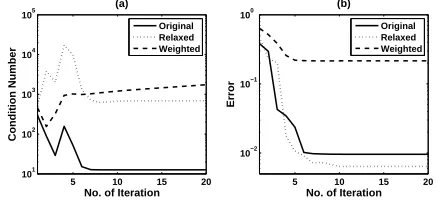
Fig. 4. (a) Condition number of the system equation matrix in (8), and (b)

L_{2 error of the approximation using original VF (6), relaxed VF (16) and}

weighted VF.

macromodel for a linear-phase (time-delayed) response, L2

approximation gives a more accurate macromodel for a noisy response, andL1approximation is favorable for system

iden-tification with an impulsive-noise-contaminated signal.

VIII. NUMERICALEXAMPLES

The VF is coded in Matlab m-script files and run in the Matlab 7.5 on a 1GB-RAM 3.4GHz PC. The example arises from a power distribution network of an IC power plane [2], whose admittance responses range from DC to 9GHz. The port response is fitted using relaxed VF [19] with a 35th-order macromodel with 10 iterations (18.28 seconds) and a set of linear-spaced initial poles, which gives 0.0064L2 and

0.0022L∞error in fitting. Fig. 3 plots the magnitude-domain responses of the converged approximant. Fig. 4 shows the condition number of the system equation matrix (8) and theL2

error during iterations. In general, VF converges quickly (≤10 iterations), especially for minimum-phase (passive) response. For further analysis of generalizations of VF, we repeat the example using VF without relaxed constraint and relaxed VF with a inverse-magnitude weighting. The quantitative compar-ison is shown in Fig. 4. It shows that the weighting does not contribute much to the numerical condition, but it affects the convergence. The relaxation may affect the numerical condition of the calculation, but it also significantly improves the accuracy of the approximation. At last, we repeat the example under an SNR of -35dB. In this case, relaxed VF

[image:5.612.326.544.256.356.2]

converges with 0.0193 L2 and 0.0014 L∞ error. This shows the relaxed VF is robust to the noisy response approximation. The responses are also fitted usingL∞norm approximation with the same configuration and clean signal, which gives an approximation with 0.0165L2error and 0.0016L∞error. The magnitude-domain response of the converged approximation in Fig. 3 shows thatL∞-norm approximation renders a more accurate low-frequency (near DC) approximation which is important for simulation, and P-norm approximation can be used as an alternative approximation criterion.

IX. CONCLUSIONS

By applying a partial fraction basis, Vector Fitting (VF) has demonstrated its numerical robustness in broadband system identification. The good performance and versatile extensibil-ity of VF render it an attractive tool for signal/power integrextensibil-ity analyses. In this paper, different issues related to VF have been discussed for obtaining a good macromodel for simulation. Furthermore, aP-norm approximation criterion is proposed to provide an alternative measure to meet different requirements.

ACKNOWLEDGMENTS

The work was supported in part by the Hong Kong Research Grants Council (HKU 718509E and HKU 717407E) and the University Research Committee of The University of Hong Kong.

REFERENCES

[1] B. Gustavsen and A. Semlyen, “Rational approximation of frequency domain responses by vector fitting,” IEEE Trans. Power Delivery, vol. 14, no. 3, pp. 1052–1061, July 1999.

[2] M. Swaminathan and A. E. Engin, Power Integrity Modeling and Design

for Semiconductors and Systems, Prentice Hall PTR, 2007.

[3] N. Wong and C. U. Lei, “IIR approximation of FIR filters via discrete-time vector fitting,” IEEE Trans. Signal Process., vol. 56, no. 3, pp. 1296–1302, Mar. 2008.

[4] C. U. Lei and N. Wong, “IIR approximation of FIR filters via discrete-time hybrid-domain vector fitting,” IEEE Signal Process. Lett., vol. 16, no. 6, pp. 533–537, June 2009.

[5] C. U. Lei .et al, “Efficient design of arbitrary complex response continuous-time IIR filter,” in Trends in Communication Technologies

and Engineering Science. Apr. 2009, pp. 163–176, Springer.

[6] W. Zhang .et al, “Efficient power network analysis considering multido-main clock gating,” IEEE Trans. Comput.-Aided Design Integr. Circuits

Syst., vol. 28, no. 9, pp. 1348–1358, Sept. 2009.

[7] Y. Cai and C. Mias, “Faster 3D finite element time domain - floquet absorbing boundary condition modelling using recursive convolution and vector fitting,” IET Microwaves, Antennas and Propagation, vol. 3, no. 2, pp. 310–324, Mar. 2009.

[8] B. Gustavsen and A. Semlyen, “Simulation of transmission line transients using vector fitting and modal decomposition,” IEEE Trans.

Power Delivery, vol. 13, no. 2, pp. 605–614, Apr. 1998.

[9] D. Deschrijver, B. Haegeman, and T. Dhaene, “Orthonormal vector fitting: A robust macromodeling tool for rational approximation of frequency domain responses,” IEEE Trans. Adv. Packag., vol. 30, no. 2, pp. 216–225, May 2007.

[10] D. Deschrijver, B. Gustavsen, and T. Dhaene, “Advancements in iterative methods for rational approximation in the frequency domain,” IEEE

Trans. Power Delivery, vol. 22, no. 3, pp. 1633–1642, July 2007.

[11] D. Deschrijver and T. Dhaene, “A note on the multiplicity of poles in the vector fitting macromodeling method,” IEEE Trans. Microw. Theory

Tech., vol. 55, no. 10, pp. 736–741, Apr. 2007.

[12] B. Nouri, R. Achar, and M. S. Nakhla, “z_{-domain orthonormal basis}

functions for physical system identifications,” IEEE Trans. Adv. Packag., Accepted for future publication.

[13] S. Grivet-Talocia, “Package macromodeling via time-domain vector fitting,” IEEE Microwave Guided Wave Lett., vol. 13, no. 11, pp. 472– 474, Nov. 2003.

[14] C. U. Lei and N. Wong, “Efficient linear macromodeling via discrete-time discrete-time-domain vector fitting,” in Proc. Intl. Conf. on VLSI Design, Jan. 2008, pp. 469–474.

[15] T. Dhaene and D. Deschrijver, “Generalised vector fitting algorithm for macromodelling of passive electronic components,” IEE Electronics

Letters, vol. 41, no. 6, pp. 299–300, Mar. 2005.

[16] L. De Tommasi, D. Deschrijver, and T. Dhaene, “Transfer function identification from phase response data,” AEU International Journal of

Electronics and Communications, 2010, Accepted for future publication.

[17] W. Hendrickx, D. Deschrijver, L. Knockaert, and T. Dhaene, “Mag-nitude vector fitting to interval data,” Mathematics and Computers in

Simulation, vol. 80, no. 3, pp. 572–580, Nov. 2009.

[18] N. Stevens, D. Deschrijver, and T. Dhaene, “Fast automatic order estimation of rational macromodels for signal integrity analysis,” in

Proc. IEEE Workshop on Signal Propagation on Interconnects, May

2007, pp. 89–92.

[19] B. Gustavsen, “Improving the pole relocating properties of vector fitting,” IEEE Trans. Power Delivery, vol. 21, no. 3, pp. 1587–1592, July 2006.

[20] B. Gustavsen and C. Heitz, “Modal vector fitting: A tool for generating rational models of high accuracy with arbitrary terminal conditions,”

IEEE Trans. Adv. Packag., vol. 31, no. 4, pp. 664–672, Nov. 2008.

[21] D. Deschrijver .et al, “Macromodeling of multiport systems using a fast implementation of the vector fitting method,” IEEE Microw. Wireless

Compon. Lett., vol. 18, no. 6, pp. 383–385, June 2008.

[22] A. Chinea, P. Triverio, and G. Grivet-Talocia, “Delay-based macromod-eling of long interconnects from frequency-domain terminal responses,”

IEEE Trans. Adv. Packag., Accepted for future publication.

[23] P. Triverio, S. Grivet-Talocia, and M. S. Nakhla, “A parameterized macromodeling strategy with uniform stability test,” IEEE Trans. Adv.

Packag., vol. 32, no. 1, pp. 205–215, Feb. 2009.

[24] R. Chakraborty, A. V. Sathanur, and V. Jandhyala, “Active-passive co-synthesis of multi-gigahertz radio frequency circuits with broadband parametric macromodels of on-chip passives,” in Proc. Intl. Conf.

Computer Aided Design, Nov. 2009, pp. 759–766.

[25] D. Deschrijver, Broadband Macromodeling of Linear Systems by Vector

Fitting, PhD dissertation, University of Antwerp, Belgium, 2008.

[26] P. Triverio, Self Consistent, Efficient and Parametric Macromodels for High-speed Interconnects Design, PhD dissertation, Politecnico di

Torino, Italy, 2009.

[27] “Official website of vector fitting,” http://www.energy.sintef.no/produkt/VECTFIT/.

[28] “Official website of IdemWorks,” http://www.idemworks.com/. [29] Official website of MATLAB RF toolbox,

http://www.mathworks.com/products/rftoolbox/.

[30] “Official website of Ansoft Nexxim,” http://www.ansoft.com/products/hf/nexxim/.

[31] R. Achar and M. S. Nakhla, “Simulation of high-speed interconnects,”

Proc. IEEE, vol. 89, no. 5, pp. 693–728, May 2001.

[32] R. Kumaresan, “Identification of rational transfer function from fre-quency response sample,” IEEE Trans. Aerosp. Electron. Syst., vol. 26, no. 6, pp. 925–934, Nov. 1990.

[33] C. Sanathanan and J. Koerner, “Transfer function synthesis as a ratio of two complex polynomials,” IEEE Trans. Autom. Control, vol. 8, no. 1, pp. 56–58, Jan. 1963.

[34] K. Steiglitz and L. E. McBride, “A technique for the identification of linear systems,” IEEE Trans. Autom. Control, vol. 10, no. 4, pp. 461– 464, Jan. 1965.

[35] P. Triverio and S. Grivet-Talocia, “Robust causality characterization via generalized dispersion relations,” IEEE Trans. Adv. Packag., vol. 31, no. 3, pp. 579–593, Aug. 2008.

[36] P. Triverio, S. Grivet-Talocia, M. S. Nakhla, F. Canavero, and R. Achar, “Stability, causality, and passivity in electrical interconnect models,”

IEEE Trans. Adv. Packag., vol. 30, no. 4, pp. 795–808, Nov. 2007.

[37] S. Grivet-Talocia and A. Ubolli, “A comparative study of passivity enforcement schemes for linear lumped macromodels,” IEEE Trans.

Adv. Packag., vol. 31, no. 4, pp. 673–683, Nov. 2008.

[38] T. Palenius and J. Roos, “Comparison of reduced-order interconnect macromodels for time-domain simulation,” IEEE Trans. Microw. Theory

Tech., vol. 52, no. 9, pp. 2240–2250, Sept. 2004.