A Method For Fitting A
p
RARMAX Model: An Application
To Financial Data
Marta Ferreira and Lu´ısa Canto e Castro
∗Abstract—Ferreira and Canto e Castro [6] introduces a power
max-autoregressive process, in short pARMAX, as an
alterna-tive to heavy tailed ARMA. An extension ofpARMAX was
con-sidered in Ferreira and Canto e Castro [7], by including a
ran-dom component, and hence calledpRARMAX, which makes the
model more flexible to applications. It was then developed a methodology settled on minimizing the Bayes risk in classifica-tion theory, but only considering standard uniform random
com-ponents. We now extend this procedure to the more generalBeta
distribution. We illustrate the method with an application to a financial data series. In order to improve estimates of the ex-ceedance probabilities of levels of interest, we use Bortot and Tawn [2] approach and derive a threshold-dependent extremal index which relates with the coefficient of tail dependence of
Led-ford and Tawn [8] and with thepRARMAX parameter.
Keywords: Extreme value theory, max-autoregressive models, clas-sification theory, Bayes error
1
Introduction
The Extreme Value Theory (EVT) has been increasingly used in areas such as finance, insurance, engineering, geophysics and telecommunications, due to the growing interest in the possibility of occurrence and impact of extreme events and the need to take them into account in modeling. Initially it was sustained in observations considered independent and identically distributed (i.i.d.), but recently, models for ex-treme values have been constructed under the more realis-tic assumption of temporal dependence. Among these, sta-tionary Markov chains are very interesting, in particular the max-autoregressive ones due to a somewhat simple treatment with regard to extremal properties. The MARMA (
max-autoregressive moving average) processes presented in Davis
and Resnick [4], in particular the ARMAX or MARMA(1,0) (Alpuim [1]), and their generalizations have applications in various phenomena, e.g., priority queues [4], accumulation of solar energy [3] and financial series [10].
In modeling dependence, it is important to assess if there is asymptotic tail independence (i.e., a dependence that gradually disappears at more and more extreme levels) or exact dependence. Ledford and Tawn [8] have proposed a model with a new parameter, usually denoted η, that measures the “degree” of tail dependence, known as
coef-∗31 March 2010; University of Minho, /DMAT-CMAT, Braga - Portugal
Email: [email protected] & Faculdade de Ciˆencias da Universi-dade de Lisboa/DEIO-CEAUL, Lisboa - Portugal Email: [email protected]
ficient of asymptotic tail dependence. When computing η
for the above mentioned MARMA, another class of max-autoregressive processes arises: the power max-max-autoregressive
pARMAX, which includes a power parameter c
(0<c<1), that is related with η (Ferreira and Canto e Castro [6]). More precisely, we haveη =max(1/2,c)and hence, as 1/2 ≤η <1, the process is asymptotically tail independent with positive association. There are several estimators forη with good properties (see, for instance [8]) and this allows us to obtain good estimates for the model parameterc. In order to make the pARMAX process more applicable to real data, it is considered a generalized version by including a random factor, denoted pRARMAX. More precisely, a sequence{Xi}i∈ZispRARMAX, if
Xi=UiXic−1∨Zi, 0<c<1,i∈Z, (1)
where{Zi}i∈Z and{Ui}i∈Z are i.i.d. r.v.’s and independent of
each other (ifU=1 we obtain pARMAX). For pRARMAX the same connection between the power parametercandη holds. A sufficient condition for stationarity is to consider innovations{Zi}i∈Z in the Fr´echet max-domain of attraction,
which in turn leads to an unit extremal index, i.e.,θ=1. See Ferreira and Canto e Castro [7] for details.
Example: Consider Z such that, FZ(x) =
1−x−1/γ
1−(B(1
cγ+p,q)/B(p,q))x−1/(cγ)
1{x≥1}, where B(p,q) is the
Eu-ler Beta function, and U Beta(p,q), p,q >0. Then,
K(x) = 1−x−1/γ1
{x≥1}, is non-degenerate stationary
distribution ofXi.
Another interesting feature of pRARMAX is that, because of an asymptotically tail independent behavior jointly with an unit extremal index, it presents a thinning of clusters of extremes as the threshold increases, until exceedances occur singly. In such cases, there is an advantage (for inferential purposes) ifθis replaced by a pre-asymptotic extremal index on the approximation,
Pn
i=1Yi≤q
≈P(Y1≤q)nθ, (2)
for largenandq. Based on Bortot and Tawn [2] approach, we consider a threshold-dependent extremal index,
1−θ(u)∼(t(u))1−1/ηL(t(u)), witht(u) = (1−K(u))−1, (3)
given byη=max(1/2,c), hence relates with model parame-terc. More precisely, approximation (3) is a consequence of having
∑rn
j=3P(X1>un,
j−1
i=2Xi≤un,Xj>un)
P(X1>un,X2>un) →0,asn→∞,
where (un)n is a real sequence such that n(1−K(un))→
τ >0, and (rn)n≥1 a nondecreasing integer sequence with
rn=o(n), asn→∞. In addition, we have that,P(
n
i=1Xi≤
un)−Kn(un) =O
n1−1/cL(
a1τ//cn)
, whereL is some slowly varying function, and also, P(ni=1Xi≤un)−Knθ(un)(un) =
on1−1/cL(a1/c
τ/n)
, withθ(u)≡θ(u,r[u])given in (3). There-fore, replacing the unitθ byθ(u)in approximation (2) leads to an improvement of this latter. For details, see Ferreira and Canto e Castro [7].
Making use ofpRARMAX flexibility, a methodology for as-sessing the adjustment of this model to real data was devel-oped in [7]. This procedure is based on minimizing the Bayes risk in classification theory and it had been only considered forUiU(0,1). In this paper, we will show that it easily
extends to UiBeta(p,q), p,q >0 (includes U(0,1)). The
method is applied to a financial series (S&P500log-returns) and we conclude for the goodness-of-fit of the model. We estimate exceeding probabilities of high levels considered as risky amounts.
2
How to fit a
pRARMAX model
In the following, we present a summary of the method. For details, see Ferreira and Canto e Castro [7]. ThepRARMAX is a suitable model for any given observed time series{Xi}i∈Z, ifXi=max(UiXic−1,Zi), that is, eachXieither comes from the
first component or from the second component of the maxi-mum. ConsideringG0the set ofXi’s that come from the
sec-ond component (Zi), andG1 the set ofXi’s coming from the
first component (UiXic−1), we will say that the model fits if, for
the observations inG0the assumptions considered forZ are not rejected, and for the observations inG1, when divided by
Xc
i−1, the hypotheses assumed forU are not rejected, as well.
So we need to classify each observation as belonging toG0or
G1. IfXi≥Xic−1, obviouslyXi∈G0, but the caseXi<Xic−1
re-quires a rule-making, which has four possible outcomes with two of them being misclassifications that will be penalized. We applyclassification theorybased on a Bayesian solution that minimizes the risk of possible wrong decisions and this is conducted in an hypothesis tests context as in Storey [9]. Ta-ble 1 summarizes the procedure and lead us to the settlement of theBayes errorgiven by
BE(Γ) = (1−λ)P(T∈Γ,H=0) +λP(T∈Γ,H=1) (4)
whereΓis the significance region of the associated hypothesis tests. None of the errors (type I or II) is fixed in advance, they can take any value as long asBE(Γ)is minimum. Assuming
Xi|Xi<Xic−1,Hi (1−Hi)·F0+Hi·F1,F0andF1are the d.f.’s of
the r.v.’s inG0and inG1, respectively, with densitiesf0andf1,
the significance region
Bλ=t:π0f0(t)/(π0f0(t) +π1f1(t))≤λ
, (5)
withP(H=1) =π1=1−π0, minimizes theBayes errorin
(4), for eachλ (0≤λ≤1). Since our decision criterion only respects,Xi<Xic−1, we need to compute,
P(Xi≤x|Xi<Xic−1) =
P(Xi≤x,Xi<Xic−1)
P(Xi<Xic−1) =
F1(x) +F0(x)
P(Xi<Xic−1),
(6)
withF1(x)=P(Xi≤x,Xi<X c i−1,UiX
c
i−1>Zi)andF0(x)=P(Xi≤
x,Xi<X
c i−1,UiX
c
i−1≤Zi). For each fixed λ, we determine the
significance region,Bλ, defined in (5). In the following, we illustrate the calculations for the modelpRARMAX of exam-ple above, where now the r.v.U isBeta(p,q), p,q>0. We have successively,
F1(x) =
1
0
x
1
Puz1c<X
n−1≤
x
u
1
cdF
Z(z)dFU(u)
=E(Uγ1c)
x
1
z−γ1cdF
Z(z)−x− 1 cγFZ(x) ,
F0(x) =
1
0
x
1
Pz1/c<X
n−1<
z
u
1/c
dFZ(z)dFU(u)
=E
U1/(γc) cγ
x
1 z
−1/(cγ)f Z(z)dz,
f1(x) =E(U1cγ/(γc))x−1/(cγ)−1F
Z(x)
and
f0(x) =E(U
1/(γc))
cγ x−
1/(cγ)f
Z(x).
In what concerns,π1=P(H=1) =P(Xi∈G1|Xi<Xic−1), we
have that,
π1 =
P(UiXic−1>Zi)
P(Xc
i−1>Zi)
=
1
0
∞
1(z/u)−1/(γ
c)dF
Z(z)dFU(u)
∞
1 z−1/(γc)dFZ(z)
=EU1/(γc)
(7)
Therefore, with π0=1−π1, the significance region (5) is
given by,
Bλ =
t: π0t
−1/(cγ)f
Z(t)
(π0t−1/(cγ)f
Z(t) + (1−π0)t−1/(cγ)−1FZ(t))
≤λ
. (8)
Note that r.v.U in this context has distribution Beta condi-tional onXi=UiXic−1and on the criterionUiXic−1>tλ, where tλ is the critical value obtained in (8). Thus being,
P(Ui≤u|UiXic−1>tλ,Xi=UiXic−1)
=
∞
1
∞
1 P
tλ
xc∨xzc <Ui≤u
dFZ(z)dK(x)
∞
1
∞
1
PUi>txλc∨xzc
dFZ(z)dK(x)
, (9)
where, for the numerator, and takingA= (tλ/u)1/c, we obtain,
∞
A
FU(u)FZ(uxc)dK(x)−
∞
A
tλ
1
FU(
tλ
xc)dFZ(z)dK(x)
− ∞
A
uxc
tλ
FU(xzc)dFZ(z)dK(x).
PUn≤u|UnXnc−1>tλ,Xn=UnXnc−1
=1
I
∞
A
x−c
uxc
tλ
fU(z/xc)FZ(z)dzdK(x)
where,I=∞
t1/c
λ
xc
tλfU(z/xc)FZ(z)dz
dK(x). Hence the density function is given by,
1
I
∞
A
fU(u)FZ(uxc)dK(x)
= u1/(cγ)+p−1(1−u)q−1
B(p,q)cγI
∞
tλ
FZ(y)y−1/(cγ)−1dy.
(10)
Therefore, the r.v.’sUicaptured by the criterion areBeta
p+
1
cγ,q
distributed. Here is a summary of the steps to fit a
pRARMAX model to a time series data:
1. Test if the given sample, X= (X1,X2,...,Xn), is in the
Fr´echet max-domain of attraction and estimate the tail index, here denotedγX(e.g., Hill estimator);
2. Estimate parametercof modelpRARMAX through the estimation of η which is the tail index (γT) of T(n) =
(T1(n),...,T
(n)
n−1), with T
(n)
i =min
n+1
n+1−Ri,
n+1
n+1−Ri+1
, i=
1,...,n, whereRiis the rank ofXiamong(X1,...,Xn);
3. Based on the criterion: “ifXi>Xic−1(c=γT, obtained in
step 2.) thenXi=Zi”, separate the innovations,Z, and
test if this sample is also in the Fr´echet max-domain of attraction;
4. Capture the observations corresponding toU, through the criterion: “ifXi<Xic−1andXi∈Bλgiven in (8), whereγX
andcare the estimates obtained in steps 1. and 2., respec-tively, then,Ui=Xi/Xic−1”;λ must be chosen in order to
minimize the Bayes error in (4) but also allowing to cap-ture a reasonable number of “true values” ofU(30);
5. Test whether the sample of r.v.’sU captured in the pre-vious step has distributionBeta(1/(γXc) +p,q)(use, for
[image:3.595.302.540.206.274.2]instance, the Kolmogorov-Smirnov test).
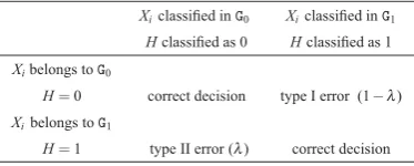
Table 1:Possible outcomes of a classification criterion along with an inter-pretation under an hypothesis test procedure with misclassification penalties
λ.
Xiclassified inG0 Xiclassified inG1
Hclassified as 0 Hclassified as 1
Xibelongs toG0
H=0 correct decision type I error (1−λ)
Xibelongs toG1
H=1 type II error (λ) correct decision
2.1
An application to financial data
In financial markets often one has to decide on a big risky in-vestment while cannot afford to have a loss larger than a cer-tain amount. Hence, it may be of interest to know the proba-bility that the maximum volatility exceeds that amount of risk.
We will see that apRARMAX process with Pareto marginals and random components, UU(0,1), performs quite well in modeling the volatility of S&P500 stock market index, through the implementation of the procedure outlined above. More precisely, we examine the square of the log-returns
Ri=logPi+1/Pi, 1≤i≤n−1 (“volatility” can be measured
through|Ri|or, equivalently,R2i), wherePi denotes the index
calculated at the end of theith trading day in the years 1957 to 1987, amounting a sample sizen=7733. The series {Ri}i
and{R2
i}i are plotted in Figure 1, in which the large peak
corresponds to Monday stock market crash on the 19th Oc-tober 1987, known as “Black Monday”. According to step
19571958 196019621963 19651966 196819701971 19731974 197619781979 198119821984 19861987 -0,25
-0,2 -0,15 -0,1 -0,05 0 0,05 0,1 0,15
0 1000 2000 3000 4000 5000 6000 7000 8000 0
0.005 0.01 0.015 0.02 0.025 0.03 0.035 0.04 0.045 0.05
0 200 400 600 800 1000 1200 0
2 4 6 8 10 12 14
k
Figure 1: Daily log-returns (left), respective squares (middle) ofS&P500
stock market index and sample path of the extreme value condition test
ap-plied to the series{R2
i}i, (horizontal line: critical value above which reject
X∈D(Gγ)γ≥0).
1., we test if the data present a heavy tail. In Figure 2 (top left) the horizontal line corresponds to the critical value above which we reject the extreme value condition. Hence it is not rejected fork700. The sample path of Hill estimator (Fig-ure 2 top right) shows an upward trend, whereas the moment and maximum likelihood estimators in (bottom left and right respectively) are much more stable: from these latter we ad-vance the estimate,γX ≈0.5 (value where the paths yield an
almost flat line; the argument for this value will be further strengthened ahead). In order to obtain a data series with
stan-0 500 1000 1500 2000 2500 3000 0.4
0.5 0.6 0.7 0.8 0.9 1 1.1
k 0 500 1000 1500 2000 2500 3000 0.4
0.5 0.6 0.7 0.8 0.9 1 1.1 1.2
k
5334 756 1224 1738 2252 2766 3280 3794 4308
0.4
0.6
0.8
1.0
1.2
[image:3.595.309.538.466.531.2]Exceedances
Figure 2:Sample paths of Hill (left), moment (middle) and maximum
like-lihood estimators (right) for the squared log-returnsR2
i.
dard Pareto marginals, a robust regression was implemented leading to a scale estimate,a=13618.3, and a shift estimate,
b=1.1. Thus, our analysis focuses on the transformed data,
Xi=a R2i +b, (1≤i≤n withn=7733). From now on we
will refer to this data set as “X”.
We test again the extreme value condition which is not rejected for 165k900 as shown in Figure 3 (top left). Consider-ing the sample paths of Hill, moment and maximum likelihood estimators in Figure 3, the previous estimate,γX≈0.5, seems
[image:3.595.68.255.582.657.2]0 200 400 600 800 1000 1200 0
0.5 1 1.5 2 2.5 3
k 0 500 1000150020002500 30003500 0.4
0.5 0.6 0.7 0.8 0.9 1 1.1 1.2 1.3
k 0 500 10001500200025003000 3500
0.4 0.5 0.6 0.7 0.8 0.9 1
[image:4.595.339.501.47.189.2]k
Figure 3: Left: sample path of the extreme value condition test applied
to the transformed dataX, (horizontal line: critical value above which reject
X∈D(Gγ)γ≥0); sample paths of Hill (middle) and moment (right) forX.
0.4γX0.45.
According to step 2., we transformXintoT(n) and then es-timate parameterc through the tail index of T(n).
Observ-ing Figure 4, the estimate is about 0.85. However, due to some stability around 0.75, we consider,c=0.85,c=0.8 and
c=0.75. The innovationsZ, captured on step 3., seem also to
0 500 1000 1500 2000 25003000 3500 0.3
0.4 0.5 0.6 0.7 0.8 0.9 1 1.1 1.2 1.3
k 0 500 1000 1500 20002500 3000 3500 0.3
0.4 0.5 0.6 0.7 0.8 0.9 1 1.1 1.2 1.3
k 20 369 769 1202 1685 2168 2651 3134 3617 4100 4583
0.7
0.8
0.9
1.0
1.1
1.2
[image:4.595.39.275.49.114.2]k
Figure 4:Sample paths of Hill (left), moment (center) and maximum
like-lihood (right) estimators, of the transformed sampleT(n)fromX.
0 0,5 1 1,5 2 2,5 3
0 250 500 750 1000 1250 0.40 500 1000 1500 2000 0.5
0.6 0.7 0.8 0.9 1 1.1 1.2 1.3
k 0 500 1000 1500 2000 0.4
0.5 0.6 0.7 0.8 0.9 1 1.1
[image:4.595.41.287.260.329.2]k
Figure 5: Left: sample path of the extreme value condition test for the
innovationsZ, captured fromXon step 3.; sample paths of Hill (center) and
moment (right) estimators, forZ.
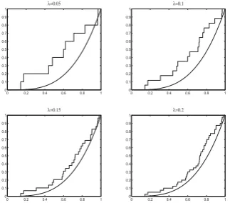
confirm a Fr´echet max-domain of attraction (Figure 5). Car-rying out step 4., we capture the observations corresponding toU, for λ = 0.05,0.1,...,0.5 and for the three scenarios (c=0.85,0.8,0.75). On step 5., we apply the Kolmogorov-Smirnov test for the distributionBeta(1/(0.5∗c) +1,1). In the case, c=0.85, rejection is obtained for λ ≥0.20 (see Figure 6) and the choice λ =0.15 matches with the sim-ulation study in Ferreira and Canto e Castro [7] (with 29 observations captured). Taking c=0.8 (less catches) then
Beta(1/(0.5∗0.8) +1,1) is rejected for λ ≥0.3 with the best fit occurring forλ =0.2, and with c=0.75 (even less catches) only rejectsBeta(1/(0.5∗0.75) +1,1)forλ =0.5, both matching once again the simulation results in Ferreira and Canto e Castro [7].
ThoughpRARMAX fits to all data set, it is actually profiled for the modeling of large values, also known asrare events. As already mentioned, we are interested in estimating the proba-bility that the maximum volatility exceeds a risky amount, for which we use the approximation in (2) considering both,θ=1 (the true value) andθ replaced by the pre-asymptotic version,
0 0.2 0.4 0.6 0.8 1 0
0.1 0.2 0.3 0.4 0.5 0.6 0.7 0.8 0.9
1 λ=0.05
0 0.2 0.4 0.6 0.8 1 0
0.1 0.2 0.3 0.4 0.5 0.6 0.7 0.8 0.9
1 λ=0.1
0 0.2 0.4 0.6 0.8 1 0
0.1 0.2 0.3 0.4 0.5 0.6 0.7 0.8 0.9
1 λ=0.15
0 0.2 0.4 0.6 0.8 1 0
0.1 0.2 0.3 0.4 0.5 0.6 0.7 0.8 0.9
1 λ=0.2
Figure 6: Empirical and theoretical d.f.’s of the random coefficients,U,
captured fromXthrough step 4. (withc=0.85), for significance regions
with,λ=0.05, ...,λ=0.20.
[image:4.595.44.284.376.443.2]θ(u) =1−u1γ(1−1/c), derived from (3). Beside estimate 0.5, we also takeγ=0.45 andγ=0.4, so we can see the effect of the very large peak. From Table 2, where we are considering the risky level 0.2, the probability estimates decrease significantly with the decrease ofγ. Yet, in what respectsc, a very small decrease takes place. Henceγis a crucial parameter. Further-more, we can also see that the higher theγand thecthe greater the differences in estimates.
Table 2: Estimates of the probability that the maximum volatility exceeds
0.2, based on (2), withθ=θ(u) =1−u1γ(1−1/c)(first 3 lines) and withθ=1
(last line), consideringn=10000.
γ=0.5 γ=0.45 γ=0.4
c=0.85 0.053222 0.010474 0.002881
c=0.8 0.057372 0.015703 0.003028
c=0.75 0.059219 0.01609 0.00308
θ=1 0.060295 0.016281 0.003101
References
[1] Alpuim, M.T., “An extremal markovian sequence,” J.
Appl. Probab., V26, pp. 219-232, 1989.
[2] Bortot, P., Tawn, J., “Models for the extremes of Markov Chains,”BiometrikaV85, pp. 851-867, 1998.
[3] Daley D., Haslet J., “A thermal energy storage with con-trolled input,”Adv. in Appl. Probab., V14, N2, pp. 257-271, 1982.
[4] Davis, R., Resnick, S, “Basic properties and prediction of max-ARMA processes,”Adv. Appl. Probab., V21, pp. 781-803, 1989.
[image:4.595.335.505.404.467.2][6] Ferreira, M., Canto e Castro, L., “Tail and dependence behaviour of levels that persist for a fixed period of time,”
Extremes,V11, pp. 113-133, 2008.
[7] Ferreira M., Canto e Castro L, “Modeling rare events through a pRARMAX process,”Notas e Comunicac¸˜oes
do CEAUL, 03/09.
[8] Ledford, A., Tawn, J.A., “Statistics for near indepen-dence in multivariate extreme values,”Biometrika, V83, pp. 169-187, 1996.
[9] Storey, J.D., “The Positive False Discovery Rate: A Bayesian Interpretation and theq-Value,”Ann. Statist., V31, pp. 2013-2035, 2003.
[10] Zhang, Z., Smith, R.L., “Modelling Financial Time
Series Data as Moving Maxima Processes”, Tech.
Rep. Dept. Stat. (Univ. North Carolina, Chapel
Hill, NC, 2001); http://www.stat.unc.edu/faculty/rs/