Learning the Structure of Variable Order CRFs: a finite state perspective

Learning the Structure of Variable-Order CRFs: a Finite-State

Perspective

Thomas Lavergne and François Yvon

LIMSI, CNRS, Univ. Paris-Sud, Université Paris Saclay Campus Universitaire, F-91 403 Orsay, France

{lavergne,yvon}@limsi.fr

Abstract

The computational complexity of linear-chain Conditional Random Fields (CRFs) makes it difficult to deal with very large label sets and long range dependencies. Such situations are not rare and arise when dealing with morphologically rich languages or joint labelling tasks. We ex-tend here recent proposals to consider vari-able order CRFs. Using an effective finite-state representation of variable-length de-pendencies, we propose new ways to per-form feature selection at large scale and re-port experimental results where we outper-form strong baselines on a tagging task.

1 Introduction

Conditional Random Fields (CRFs) (Lafferty et al., 2001; Sutton and McCallum, 2006) are a method of choice for many sequence labelling tasks such as Part of Speech (PoS) tagging, Text Chunking, or Named Entity Recognition. Linear-chain CRFs are easy to train by solving a convex optimization problem, can accomodate rich fea-ture patterns, and enjoy polynomial exact infer-ence procedures. They also deliver state-of-the-art performance for many tasks, sometimes surpass-ing seq2seq neural models (Schnober et al., 2016). A major issue with CRFs is the complexity of training and inference procedures, which are quadratic in the number of possible output la-bels for first order models and grow exponen-tially when higher order dependencies are consid-ered. This is problematic for tasks such as precise PoS tagging for Morphologically Rich Languages (MRLs), where the number of morphosyntactic la-bels is in the thousands (Hajiˇc, 2000; Müller et al., 2013). Large label sets also naturally arise when joint labelling tasks (eg. simultaneous PoS

tag-ging and text chunking) are considered, For such tasks, processing first-order models is demanding, and full size higher-order models are out of the question. Attempts to overcome this difficulty are based on a greedy approach which starts with first-order dependencies between labels and iteratively increases the scope of dependency patterns under the constraint that a high-order dependency is se-lected only if it extends an existing lower order feature (Müller et al., 2013). As a result, fea-ture selection may only choose only few higher-order features, motivating the need for an effec-tive variable-order CRF (voCRF) training proce-dure (Ye et al., 2009).1 _{The latest implementation} of this idea (Vieira et al., 2016) relies on (struc-tured) sparsity promoting regularization (Martins et al., 2011) and on finite-state techniques, han-dling high-order features at a small extra cost (see § 2). In this approach, the sparse set of label de-pendency patterns is represented in a finite-state automaton, which arises as the result of the fea-ture selection process.

In this paper, we somehow reverse the perspec-tive and consider VoCRF training mostly as an au-tomaton inference problem. This leads us to con-sider alternative techniques for learning the finite-state machine representing the dependency struc-ture of sparse VoCRFs (see § 3). Two lines of enquiries are explored: (a) to take into account the internal structure of large tag sets in order to learn better and/or leaner feature sets; (b) to de-tect unconditional structural dependencies in label sequences in order to speed-up the discovery of useful features. These ideas are implemented in6 feature selection strategies, allowing us to explore a large set of dependency structures. Relying on lazy finite-state operations, we train VoCRFs up to order 5, and achieve PoS tagging performance that 1_{This is reminiscent ofvariable order HMMs, introduced} eg. in (Schütze and Singer, 1994; Ron et al., 1996).

surpass strong baselines for two MRLs (see § 4).

2 Variable order CRFs

In this section, we recall the basics of CRFs and VoCRFs and introduce some notations.

2.1 Basics

First-order CRFs use the following model:

pθ(y|x) =Zθ(x)−1exp(θTF(x,y)) (1)

wherex= (x1, . . . , xT)andy= (y1, . . . , yT)are the input (in XT_{) and output (in Y}T_{) sequences} and Zθ(x) is a normalizer. Each component Fj(x,y)of the global feature vector decomposes as a sum of local features PT_t=1fj(yt−1, yt, xt) and is associated to parameterθj. Local features typically use binary tests and take the form:

fu,g(yt−1, yt, x, t) =I(yt=u∧g(x, t)) fuv,g(yt−1, yt, x, t) =I(yt−1yt=uv∧g(x, t))

whereI()is an indicator function andg()tests a local property ofxaroundxt. In this setting, the number of parameters is|Y|2_{× |X |train, where|A|}

is the cardinality of A and|X |train is the number of values of g(x, t) observed in the training set. Even in moderate size applications, the parameter set can be very large and contain dozen of millions of features, due to the introduction of sequential dependencies in the model.

Given N i.i.d. sequences {x(i)_,y(i)_}N

i=1,

esti-mation is based on the minimization of the negated conditional log-likelihood l(θ). Optimizing this objective requires to compute its gradient and to repeatedly evaluate the conditional expectation of the feature vector. This can be done using a forward-backward algorithm having a complexity that grows quadratically with |Y|. l(θ) is usu-ally complemented with a regularization term so as to avoid overfitting and stabilize the optimiza-tion. Common regularizers use the`1- or the`2

-norm of the parameter vector, the former having the benefit to promote sparsity, thereby perform-ing automatic feature selection (Tibshirani, 1996).

2.2 Variable order CRFs (VoCRFs)

When the label set is large, many pairs of labels never occur in the training data and the sparsity of label ngrams quickly increases with the orderp of the model. In the variable order CRF model, it is assumed that only a small number of ngrams

Algorithm 1:BuildingA[W]

W :list of patterns,A[W]initially empty

U =Pref(W)

foreachw∈ Wdo

TrieInsert(w, A[W])

//Add missing transitions

foreachu=vy∈ U do

new FailureTrans(u,LgSuff(v,U))

(out of|Y|p_{) are associated with a non-zero} param-eter value. Denoting W the set of such ngrams and w ∈ W, a generic feature function is then fw,g(w, x, t) =I(yt−s. . . yt=w∧g(x, t)).

In (order-p) VoCRFs, the computational cost of training and inference is proportional to the size of a finite-state automaton A[W]encoding the pat-terns in W,2 _{which can be much less than |Y|}p_. Our procedure for building A[W] is sketched in Algorithm 1, whereTrieInsertinserts a string in a trie, Pref(W) computes the set of prefixes of the strings in W,3 _{LgSuff(v,U) returns the} longest suffix of v in U, and FailureTrans is a special ε-transition used only when no la-belled transition exists (Allauzen et al., 2003).4 Each state (or pattern prefix) v inA[W]is asso-ciated with a set of feature functions{fu,g,∀u ∈ Suff(v), g}.5 _{The forward step of the gradient} computation maintains one valueα(v, t)per state and time step, which is recursively accumulated over all paths ending invat timet.

The next question is to identify W. The sim-plest method keeps all the ngrams viewed in train-ing, additionally filtering rare patterns (Cuong et al., 2014). However, frequency based feature se-lection does not take interactions into account and is not the best solution. Ideally, one would like to train a complete order-p model with a sparsity promoting penalty, a technique that only works for small label sets.6 _{The greedy algorithm of}

2_{More precisely, Vieira et al. (2016) considerW, the} clo-sure ofWunder suffix and last character substitution, which factors asW=H × Y. The complexity of training depends on the size of the finite-state automaton representingW.

3_{A trie has one state for each prefix.}

4_{This was also suggested by Cotterell and Eisner (2015)} as a way to build a more compact pattern automaton.

5_{Upon reaching a statev, we need to access the features} that fire for that pattern, and also for all its suffixes. Each state thus stores a set of pattern; each pattern is associated with a set of tests on the observation (cf. 2.1).

Schmidt and Murphy (2010); Vieira et al. (2016) is more scalable: it starts with all unigram patterns and iteratively growsW by extending the ngrams that have been selected in the simpler model. At each round of training, feature selection is per-formed using a`1 penalty and identifies the

pat-terns that will be further augmented.

3 Learning patterns

We introduce now several alternatives for learning

W. Our motivation for doing so is twofold: (a) to take the internal structure of large label sets into account; (b) to identify more abstract patterns in label sequences, possibly containing gaps or iter-ations, which could yield smaller A[W]. As dis-cussed below, both motivations can be combined.

3.1 Greedy`1

The greedy strategy iteratively grows patterns up to order p. Considering all possible unigram and bigram patterns, we train a sparse model to select a first set of useful bigrams. In subsequent iter-ations, each pattern w selected at order k is ex-tended in all possible ways to specify the pattern set at orderk+ 1, which will be filtered during the next training round. This approach is close, yet simpler, than the group lasso approach of Vieira et al. (2016) and experimentally yields slightly smaller pattern sets (see Table 2). This is because we do not enforce closure under last-character re-placement: once patternw is pruned, longer pat-terns ending inware never considered.7

3.2 Component-wise training

Large tag sets often occur in joint tasks, where multiple levels of information are encoded in one compound tag. For instance, the fine grain labels in the Tiger corpus (Brants et al., 2002) combine PoS and morphological information in tags such asNN.Dat.Sg.Femfor a feminine singular da-tive noun. In the sequel, we refer to each piece of information as a tag component. We assume that all tags contain the same components, using a “non-applicable” value whenever needed. Us-ing features that test arbitrary combinations of tag components would make feature selection much more difficult, as the number of possible patterns grows combinatorially with the number of compo-nents. We keep things simple by allowing features to only evaluate one single component at a time:

7_{cf. the discussion in (Vieira et al., 2016, § 4).}

this allows us to identify dependencies of different orders for each component.

Assuming that each tag y containsK compo-nentsy = [z1, z2. . . , zK], withzk ∈ Yk, W is then computed as in § 3.1, except that we now con-sider one distinct set of patternsWkfor each com-ponentk. At each training round, each set Wkis extended and pruned independently from the oth-ers. Note that all these automata are trained simul-taneously using a common set of features. This process results in K automata, which are inter-sected on the fly8 _{using “lazy” composition. In} our experiments, we also consider the case where we additionally combine the automaton represent-ing complete tag sequences: this has the benefi-cial effect to restrict the combinations of subtags to values that actually exist in the data.

3.3 Pruned language models

Another approach for computingW assumes that useful dependencies between tags can be iden-tified using an auxiliary language model (LM) trained without paying any attention to observa-tion sequences. A patternw will then be deemed useful for the labelling task only ifw is a useful history in a LM of tag sequences. This strategy was implemented by first training a compact p -gram LM with entropy pruning9 _{(Stolcke, 1998)} and including all the surviving histories inW. In a second step, we train the complete CRF as usual, with all observation features and`1penalty to

fur-ther prune the parameter set.

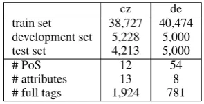
cz de

train set 38,727 40,474 development set 5,228 5,000 test set 4,213 5,000

# PoS 12 54

# attributes 13 8

# full tags 1,924 781 Table 1: Corpus description

3.4 Maximum entropy language models

Another technique, which combines the two pre-vious ideas, relies on Maximum Entropy LMs

8_{Formally, eachA[W}

k]has transitions labelled with

ele-ments ofYk; lazy intersection operates on “generalized”

tran-sitions, where each labelzis replaced with[?, . . . , z, . . . ,?], where ? matches any symbol. A[W] is the intersection T

k₉A[Wk]and is labelled with completely specified tags.

(MELMs) (Rosenfeld, 1996). MELMs decom-pose the probabililty of a sequencey1. . . yT using the chain rule, where each termpλ(yt|y<t)is a lo-cally normalized exponential model including all possible ngram features up to orderp:

p(yt|y<t;λ) =Z(λ)−1expλTG(y1. . . yt)

In contrast to globally normalized models, the complexity of training remains linear wrt.|Y|, ir-respective ofp. It it also straightforward both to (a) use a `1 penalty to perform feature selection;

(b) include features that only test specific compo-nents of a complex tag. For an orderpmodel, our feature functions evaluate alln-grams (forn≤p) of complete tags or of one specific component:

Gw(y1, . . . , yt) =I(yt−n+1. . . yt=w) Gu(y1, . . . , yt) =I(zk,t−n+1. . . zk,t=u)

Once a first round of feature selection has been performed,10 _{we compute A[W] as explained} above. The last step of training reintroduces the observations and estimates the CRF paramaters. A variant of this approach adds extragappyfeatures to the n-gram features. Gappy features at order ptest whether some labelu occurs in the remote past anywhere between positiont−p+ 111 _and t−n. They take the following form:

Gw,u(y1, . . . , yt) =I(yt−n+1. . . yt=w∧ u∈ {yt−p+1. . . yt−n}),

and likewise for features testing components.

4 Experiments 4.1 Training protocol

The following protocol is used throughout: (a) identifyW(§3) - note that this may imply to tune a regularization parameter; (b) train a full model (in-cluding tests on the observations for each pattern inW) using`1 regularization and a very small`2

term to stabilize convergence. The best regulariza-tion in (a) and (b) is selected on development data and targets either perplexity (for LMs) or label ac-curacy (for CRFs).

10_{As the LM building step only look at labels, we tune} the regularization to optimize the perplexity of the LM on a development set.

11_{We usep= 6in our experiments.}

4.2 Datasets and Features

Experiments are run on two MRLs: for Czech, we use the CoNLL 2009 data set (Hajiˇc et al., 2009) and for German, the Tiger Treebank with the split of Fraser et al. (2013)). Both datasets include rich morphological attributes (cf. Table 1).

All the patterns inW are combined withlexical features testing the current word xt, its prefixes and suffixes of length 1 to 4, its capitalization and the presence of digit or punctuation symbols. Ad-ditional contextual features also test words in a lo-cal window around positiont. These tests greatly increase the feature count and are not provided for all label patterns: for unigram patterns, we test the presence of all unigrams and bigrams of words in a window of 5 words; for bigrams patterns we only test for all unigrams in a window of 3 words. Con-textual features are not used for larger patterns.

4.3 Results

We consider several baselines: Maxent and MEMM models, neither of which considers la-bel dependencies in training, a linear chain CRF12 and our own implementation of the group lasso of Vieira et al. (2016). For the latter, we contrast two setups: one where each pattern inW gives rise to one single feature, and one where it is conjoined with tests on the observation.13 _{All scores in} Ta-ble 2 are label accuracies on unseen test data.

As expected, Maxent and MEMM are outper-formed by almost all variants of CRFs, and their scores are only reported for completeness.Group lasso results demonstrate the effectiveness of using contextual information with high order fea-tures: the gain is≈0.7 points for both languages and all values of p. Greedy `1 achieves

accu-racy results similar to group lasso, suggest-ing that`1penalty alone is effective to select

high-order features. It also yields slighly smaller mod-els and very comparable training time across the board: indeed, greedy parameter selection strate-gies imply multiple rounds of training which are overall quite costly, due to the size of the full la-bel set. Testing individual subtags (§ 3.2) results in a slight improvement (≈+0.3) in accuracy over Greedy`1. When using an additional automata

for the full tag, we get a larger gain of≈0.6 points for Czech, slightly less for German: including a model for complete tags also prevents to

cz de

p= 2 p= 3 p= 4 p= 5 p= 2 p= 3 p= 4 p= 5

90.01% 91.12% 91.17% 91.14% 85.62% 85.84% 85.96% 86.02%

Maxent 1924 1924 1924 1924 781 781 781 781

191min 219min 286min 349min 142min 193min 252min 297min

90.96% 92.09% 92.13% 92.12% 86.48% 86.88% 87.13% 87.19%

MEMM 1924 1924 1924 1924 781 781 781 781

191min 219min 286min 349min 142min 193min 252min 297min

91.93% 86.95%

Linear Chain CRF 3.7e6 – – – 6.1e5 – – –

657min 447min

91.91% 92.27% 92.41% 86.92% 87.24% 87.48%

Group lasso 9.6e5 4.3e7 1.2e8 – 1.8e5 9.2e6 5.4e7 –

421min 1656min 3067min 305min 1134min 2101min

92.51% 92.95% 93.03% 87.48% 87.92% 87.96%

Group lasso + ctx 9.2e5 4.1e7 1.2e8 – 1.7e5 7.8e6 5.3e7 –

520min 1632min 3285min 349min 1218min 2398min

92.47% 92.94% 93.01% 87.43% 87.87% 87.96%

Greedy`1 8.4e5 4.1e7 1.1e8 – 1.7e5 7.1e6 5.0e7 –

462min 1759min 3300min 340min 1239min 2357min

92.76% 93.24% 93.36% 93.28% 87.47% 88.16% 88.26% 88.29%

Component-wise 6.2e4 2.8e5 8.2e5 3.7e6 2.4e4 7.2e4 3.7e5 1.4e6 247min 370min 1179min 2224min 173min 268min 836min 1483min Component-wise

+ Full

92.97% 93.41% 93.69% 93.65% 87.39% 88.36% 88.59% 88.60% 8.7e5 2.8e7 8.3e7 4.6e8 1.4e5 5.2e6 2.1e7 1.3e8 463min 1569min 3162min 4321min 311min 1097min 2181min 3249min

92.98% 93.27% 93.51% 93.53% 87.43% 88.12% 88.25% 88.21%

Pruned LM 3.2e5 8.2e6 1.1e7 8.6e7 1.3e5 8.9e5 9.1e6 5.3e7 233min 487min 1210min 2519min 163min 372min 896min 1894min

93.02% 93.33% 93.81% 93.63% 87.41% 88.61% 88.76% 88.74%

MELM 4.6e5 1.7e7 2.3e7 1.4e8 1.4e5 2.9e6 1.4e7 9.8e7 303min 545min 1478min 2559min 206min 407min 1063min 1924min

93.52% 93.68% 93.79% 88.38% 88.70% 88.78%

MELM + Gaps 4.5e5 1.5e7 1.9e7 – 1.4e5 2.3e6 1.1e7 –

289min 658min 1751min 217min 439min 1297min

Table 2: Experimental results. Each cell reports accuracy, number of states inA[W]and total training time. Group lasso is our reimplementation of Vieira et al. (2016) (+Ctx = +context features) ; Greedy `1 is described in section 3.1, Component-wise is the decomposition approach of § 3.2, PrunedLM and

MELM (+Gaps) were described in § 3.3 and § 3.4.

ate invalid combinations of subtags. These models represent different tradeoffs between accuracy and training time: the 4-gramComponent-wise ex-periment only took 14 hrs to complete on German data and outperforms the correspondingGreedy `1setup while containing approximately 100 times

less features.Component-wise+Fullis more comparable in size and training time toGreedy `1, but yields a larger improvement in

perfor-mance. The last sets of experiments with LMs yields even better operating points, as the first stage of pattern selection is performed with a cheap model. They are our best trade-off to date, yielding the best performance for all values ofp.

5 Conclusion

In this work, we have explored ways to take advan-tage of the flexibility offered by implementations of VoCRFs based on finite-state techniques. We

have proposed strategies to include tests on sub-parts of complex tags, as well as to select useful label patterns with auxiliary unconditional LMs. Experiments with two MRLs with large tagsets yielded consistent improvements (≈+0.8 points) over strong baselines. They offer new perspectives to perform feature selection in high order CRFs. In our future work, we intend to also explore how to complement`1penalties with terms penalizing

more explicitely the processing time; we also wish to study how these ideas can be used in combina-tion with neural models.

Acknowledgements

References

Cyril Allauzen, Mehryar Mohri, and Brian Roark. 2003. Generalized algorithms for constructing sta-tistical language models. In Proceedings of the 41st Annual Meeting of the Association for Com-putational Linguistics. Association for Computa-tional Linguistics, Sapporo, Japan, pages 40–47. https://doi.org/10.3115/1075096.1075102.

Adam L. Berger, Vincent J. Della Pietra, and Stephen A. Della Pietra. 1996. A maximum entropy ap-proach to natural language processing. Comput. Linguist.22(1):39–71.

Sabine Brants, Stefanie Dipper, Silvia Hansen, Wolf-gang Lezius, and George Smith. 2002. The TIGER treebank. InProceedings of the workshop on tree-banks and linguistic theories. pages 24–41.

Ryan Cotterell and Jason Eisner. 2015. Penalized expectation propagation for graphical mod-els over strings. In Proceedings of the 2015 Conference of the North American Chapter of the Association for Computational Linguistics: Human Language Technologies. Association for Computational Linguistics, pages 932–942. https://doi.org/10.3115/v1/N15-1094.

Nguyen Viet Cuong, Nan Ye, Wee Sun Lee, and Hai Leong Chieu. 2014. Conditional Ran-dom Field with High-order Dependencies for Sequence Labeling and Segmentation. Jour-nal of Machine Learning Research 15:981–1009. http://jmlr.org/papers/v15/cuong14a.html.

Alexander Fraser, Helmut Schmid, Richárd Farkas, Renjing Wang, and Hinrich Schütze. 2013. Knowl-edge sources for constituent parsing of german, a morphologically rich and less-configurational lan-guage. CL39(1):57–85.

Jan Hajiˇc. 2000. Morphological tagging: Data vs. dic-tionaries. InProceedings of the 1st North American chapter of the Association for Computational Lin-guistics conference. Seattle, WA, pages 94–101. Jan Hajiˇc, Massimiliano Ciaramita, Richard

Johans-son, Daisuke Kawahara, Maria Antònia Martí, Lluís Màrquez, Adam Meyers, Joakim Nivre, Sebastian Padó, Jan Štˇepánek, Pavel Straˇnák, Mihai Surdeanu, Nianwen Xue, and Yi Zhang. 2009. The conll-2009 shared task: Syntactic and semantic dependencies in multiple languages. InProceedings of the Thir-teenth Conference on Computational Natural Lan-guage Learning: Shared Task. CoNLL ’09, pages 1–18.

John Lafferty, Andrew McCallum, and Fernando Pereira. 2001. Conditional random fields: Prob-abilistic models for segmenting and labeling se-quence data. In Proceedings of the 18th Interna-tional Conference on Machine Learning. Morgan Kaufmann, San Francisco, CA, Williamstown, MA, (ICML’01), pages 282–289.

Thomas Lavergne, Olivier Cappé, and François Yvon. 2010. Practical very large scale CRFs. In Pro-ceedings of the 48th Annual Meeting of the Associ-ation for ComputAssoci-ational Linguistics. Uppsala, Swe-den, pages 504–513.

Andre Martins, Noah Smith, Mario Figueiredo, and Pedro Aguiar. 2011. Structured sparsity in struc-tured prediction. InProceedings of the 2011 Con-ference on Empirical Methods in Natural Language Processing. pages 1500–1511.

Thomas Müller, Ryan Cotterell, Alexander Fraser, and Hinrich Schütze. 2015. Joint lemmatization and morphological tagging with lemming. In Proceed-ings of the 2015 Conference on Empirical Methods in Natural Language Processing. Lisbon, Portugal, EMNLP’15, pages 2268–2274.

Thomas Müller, Helmut Schmid, and Hinrich Schütze. 2013. Efficient higher-order CRFs for morpholog-ical tagging. In Proceedings of the 2013 Confer-ence on Empirical Methods in Natural Language Processing. Seattle, Washington, USA, EMNLP’15, pages 322–332.

Chris Pal, Charles Sutton, and Andrew McCal-lum. 2006. Sparse forward-backward using min-imum divergence beams for fast training of con-ditional random fields. In 2006 IEEE Interna-tional Conference on Acoustics Speech and Sig-nal Processing Proceedings. volume 5, pages V–V. https://doi.org/10.1109/ICASSP.2006.1661342. Dana Ron, Yoram Singer, and Naftali Tishby. 1996.

The power of amnesia: Learning probabilistic au-tomata with variable memory length. Machine Learning25(2-3):117–149.

Ronald Rosenfeld. 1996. A maximum entropy ap-proach to adaptive statistical learning modeling.

Computer, Speech and Language10:187 – 228. Mark W. Schmidt and Kevin P. Murphy. 2010. Convex

structure learning in log-linear models: Beyond pair-wise potentials. InProceedings of the Thirteenth In-ternational Conference on Artificial Intelligence and Statistics,. Chia Laguna Resort, Sardinia, Italy, AIS-TATS, pages 709–716.

Carsten Schnober, Steffen Eger, Erik-Lân Do Dinh, and Iryna Gurevych. 2016. Still not there? comparing traditional sequence-to-sequence models to encoder-decoder neural networks on monotone string trans-lation tasks. In Proceedings of COLING 2016, the 26th International Conference on Computational Linguistics: Technical Papers. The COLING 2016 Organizing Committee, Osaka, Japan, pages 1703– 1714.

Nobuyuki Shimizu and Andrew Haas. 2006. Exact de-coding for jointly labeling and chunking sequences. InProceedings of COLING/ACL. pages 763–770. Noah A. Smith, David A. Smith, and Roy W. Tromble.

2005. Context-based morphological disambiguation with random fields. InProceedings of Human Lan-guage Technology Conference and Conference on Empirical Methods in Natural Language Process-ing. Vancouver, British Columbia, Canada, pages 475–482.

Andreas Stolcke. 1998. Entropy-based pruning of backoff language models. InProc. DARPA Broad-cast News Transcription and Understanding Work-shop. Lansdowne, VA, pages 270–274.

Andreas Stolcke. 2002. SRILM – an extensible lan-guage modeling toolkit. InProceedings of the Inter-national Conference on Spoken Langage Processing (ICSLP). Denver, CO, volume 2, pages 901–904. Charles Sutton and Andrew McCallum. 2006. An

in-troduction to conditional random fields for relational learning. In Lise Getoor and Ben Taskar, editors,

Introduction to Statistical Relational Learning. The MIT Press, Cambridge, MA.

Robert Tibshirani. 1996. Regression shrinkage and se-lection via the lasso. Journal of the Royal Statistical Society B58(1):267–288.

Kristina Toutanova and Colin Cherry. 2009. A global model for joint lemmatization and part-of-speech prediction. In Proceedings of the Joint Confer-ence of the 47th Annual Meeting of the ACL and the 4th International Joint Conference on Natu-ral Language Processing of the AFNLP. Associa-tion for ComputaAssocia-tional Linguistics, pages 486–494. http://aclweb.org/anthology/P09-1055.

Tim Vieira, Ryan Cotterell, and Jason Eisner. 2016. Speed-accuracy tradeoffs in tagging with variable-order crfs and structured sparsity. InProceedings of the 2016 Conference on Empirical Methods in Nat-ural Language Processing. EMNLP, pages 1973– 1978.

Nan Ye, Wee S. Lee, Hai L. Chieu, and Dan Wu. 2009. Conditional random fields with high-order features for sequence labeling. In Y. Bengio, D. Schu-urmans, J. D. Lafferty, C. K. I. Williams, and A. Culotta, editors,Advances in Neural Information Processing Systems 22. Curran Associates, Inc., pages 2196–2204. http://papers.nips.cc/paper/3815-