Deeper Attention to Abusive User Content Moderation

Deeper Attention to Abusive User Content Moderation

John Pavlopoulos

Straintek, Athens, Greece

[email protected]

Prodromos Malakasiotis

Straintek, Athens, Greece

[email protected]

Ion Androutsopoulos

Athens University of Economics and Business, Greece

[email protected]

Abstract

Experimenting with a new dataset of 1.6M user comments from a news portal and an existing dataset of 115K Wikipedia talk page comments, we show that anRNN

op-erating on word embeddings outpeforms the previous state of the art in moderation, which used logistic regression or anMLP

classifier with character or wordn-grams. We also compare against a CNN

operat-ing on word embeddoperat-ings, and a word-list baseline. A novel, deep, classification-specific attention mechanism improves the performance of the RNN further, and can

also highlight suspicious words for free, without including highlighted words in the training data. We consider both fully auto-matic and semi-autoauto-matic moderation.

1 Introduction

User comments play a central role in social me-dia and online discussion fora. News portals and blogs often also allow their readers to com-ment to get feedback, engage their readers, and build customer loyalty.1 _{User comments,}

how-ever, and more generally user content can also be abusive (e.g., bullying, profanity, hate speech) (Cheng et al.,2015). Social media are under pres-sure to combat abusive content, but so far rely mostly on user reports and tools that detect fre-quent words and phrases of reported posts.2

Wul-czyn et al. (2017) estimated that only 17.9% of personal attacks in Wikipedia discussions were followed by moderator actions. News portals also

1_{See, for example,http://niemanreports.org/}

articles/the-future-of-comments/.

2 _{Consult, for example, https://www.facebook.}

com/help/131671940241729 and https://www. theguardian.com/technology/2017/feb/07/ twitter-abuse-harassment-crackdown.

suffer from abusive user comments, which dam-age their reputations and make them liable to fines, e.g., when hosting comments encouraging illegal actions. They often employ moderators, who are frequently overwhelmed, however, by the volume and abusiveness of comments.3 _{Readers are}

dis-appointed when non-abusive comments do not ap-pear quickly online because of moderation delays. Smaller news portals may be unable to employ moderators, and some are forced to shut down their comments sections entirely.

We examine how deep learning (Goodfellow et al., 2016; Goldberg, 2016, 2017) can be em-ployed to moderate user comments. We experi-ment with a new dataset of approx. 1.6M manually moderated (accepted or rejected) user comments from a Greek sports news portal (called Gazzetta), which we make publicly available.4 _{This is one}

of the largest publicly available datasets of mod-erated user comments. We also provide word em-beddings pre-trained on 5.2M comments from the same portal. Furthermore, we experiment on the ‘attacks’ dataset of Wulczyn et al. (2017), approx. 115K English Wikipedia talk page comments la-beled as containing personal attacks or not.

In a fully automatic scenario, there is no moder-ator and a system accepts or rejects comments. Al-though this scenario may be the only available one, e.g., when news portals cannot afford moderators, it is unrealistic to expect that fully automatic mod-eration will be perfect, because abusive comments may involve irony, sarcasm, harassment without profane phrases etc., which are particularly diffi-cult for a machine to detect. When moderators are available, it is more realistic to develop

semi-3_{See, e.g., https://www.wired.com/2017/04/}

zerochaos-google-ads-quality-raters and

https://goo.gl/89M2bI.

4_{The portal is http://www.gazzetta.gr/.} In-structions to download the dataset will become available at

http://nlp.cs.aueb.gr/software.html.

x

x

✓ ✓

x

x

✓ ✓

x

x

✓ ✓

✓

?

? ?

?

✓

x

Figure 1: Semi-automatic moderation.

automatic systems aiming to assist, rather than re-place the moderators, a scenario that has not been considered in previous work. In this case, com-ments for which the system is uncertain (Fig. 1) are shown to a moderator to decide; all other com-ments are accepted or rejected by the system. We discuss how moderation systems can be tuned, de-pending on the availability and workload of the moderators. We also introduce additional evalu-ation measures for the semi-automatic scenario.

On both datasets (Gazzetta and Wikipedia com-ments) and for both scenarios (automatic, semi-automatic), we show that a recurrent neural net-work (RNN) outperforms the system of Wulczyn

et al. (2017), the previous state of the art for com-ment moderation, which employed logistic regres-sion or a multi-layer Perceptron (MLP), and

rep-resented each comment as a bag of (character or word) n-grams. We also propose an attention mechanism that improves the overall performance of theRNN. Our attention mechanism differs from

most previous ones (Bahdanau et al., 2015; Lu-ong et al., 2015) in that it is used in a classifi-cation setting, where there is no previously gen-erated output subsequence to drive the attention, unlike sequence-to-sequence models (Sutskever et al.,2014). In that sense, our attention is similar to that of of Yang et al. (2016), but our attention mechanism is a deeperMLPand it is only applied

to words, whereas Yang et al. also have a second attention mechanism that assigns attention scores to entire sentences. In effect, our attention detects the words of a comment that affect most the clas-sification decision (accept, reject), by examining them in the context of the particular comment.

Although our attention mechanism does not al-ways improve the performance of theRNN, it has

the additional advantage of allowing the RNN to

highlight suspicious words that a moderator could consider to decide more quickly if a comment should be accepted or rejected. The highlighting

Dataset/Split Accepted Rejected Total G-TRAIN-L 960,378 (66%) 489,222 (34%) 1.45M G-TRAIN-S 67,828 (68%) 32,172 (32%) 100,000

G-DEV 20,236 (68%) 9,464 (32%) 29,700 G-TEST-L 20,064 (68%) 9,636 (32%) 29,700 G-TEST-S 1,068 (71%) 432 (29%) 1,500 G-TEST-S-R 1,174 (78%) 326 (22%) 1,500 W-ATT-TRAIN 61,447 (88%) 8,079 (12%) 69,526

W-ATT-DEV 20,405 (88%) 2,755 (12%) 23,160 W-ATT-TEST 20,422 (88%) 2,756 (12%) 23,178

Table 1: Statistics of the datasets used.

comes for free, i.e., the training data do not con-tain highlighted words. We also show that words highlighted by the attention mechanism correlate well with words that moderators would highlight.

Our main contributions are: (i) We release a dataset of 1.6M moderated user comments. (ii) We introduce a novel, deep, classification-specific at-tention mechanism and we show that anRNNwith

our attention mechanism outperforms the previous state of the art in user comment moderation. (iii) Unlike previous work, we also consider a semi-automatic scenario, along with threshold tuning and evaluation measures for it. (iv) We show that the attention mechanism can automatically high-light suspicious words for free, without manually highlighting words in the training data.

2 Datasets

We first discuss the datasets we used, to help ac-quaint the reader with the problem.

2.1 Gazzetta comments

There are approx. 1.45M training comments (cov-ering Jan. 1, 2015 to Oct. 6, 2016) in the Gazzetta dataset; we call themG-TRAIN-L(Table1). Some

experiments use only the first 100K comments of

G-TRAIN-L, calledG-TRAIN-S. An additional set

of 60,900 comments (Oct. 7 to Nov. 11, 2016) was split to development (G-DEV, 29,700

com-ments), large test (G-TEST-L, 29,700), and small

test set (G-TEST-S, 1,500). Gazzetta’s moderators

(2 full-time, plus journalists occasionally helping) are occasionally instructed to be stricter (e.g., dur-ing violent events). To get a more accurate view of performance in normal situtations, we manu-ally re-moderated (labeled as ‘accept’ or ‘reject’) the comments ofG-TEST-S, producingG-TEST-S -R. The reject ratio is approx. 30% in all subsets,

except forG-TEST-S-Rwhere it drops to 22%,

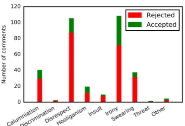
Figure 2: Re-moderated comments with at least one snippet of the corresponding category.

Each G-TEST-S-R comment was re-moderated

by five annotators. Krippendorff’s (2004) alpha was 0.4762, close to the value (0.45) reported by Wulczyn et al. (2017) for the Wikipedia ‘attacks’ dataset. Using Cohen’s Kappa (Cohen,1960), the mean pairwise agreement was 0.4749. The mean pairwise percentage of agreement (% of comments each pair of annotators agreed on) was 81.33%. Cohen’s Kappa and Krippendorff’s alpha lead to lower scores, because they account for agreement by chance, which is high when there is class im-balance (22% reject, 78% accept inG-TEST-S-R).

During the re-moderation of G-TEST-S-R, the

annotators were also asked to highlight snippets they considered suspicious, i.e., words or phrases that could lead a moderator to consider reject-ing each comment.5 _{We also asked the}

annota-tors to classify each snippet into one of the fol-lowing categories: calumniation (e.g., false accu-sations), discrimination (e.g., racism), disrespect (e.g., looking down at a profession), hooliganism (e.g., calling for violence), insult (e.g., making fun of appearance), irony, swearing, threat, other. Fig-ure2shows how many comments ofG-TEST-S-R

contained at least one snippet of each category, ac-cording to the majority of annotators; e.g., a com-ment counts as containing irony if at least 3 anno-tators annotated it with an irony snippet (not nec-essarily the same). The gold class of each com-ment (accept or reject) is determined by the ma-jority of the annotators. Irony and disrespect are particularly frequent in both classes, followed by calumniation, swearing, hooliganism, insults. No-tice that comments that contain irony, disrespect etc. are not necessarily rejected. They are, how-ever, more likely in the rejected class, consider-ing that the accepted comments are 2.5 times more

5_{Treating snippet overlaps as agreements, the mean} pair-wise Dice coefficient for snippet highlighting was 50.03%.

than the rejected ones (78% vs. 22%).

We also provide 300-dimensional word em-beddings, pre-trained on approx. 5.2M comments (268M tokens) from Gazzetta using WORD2VEC

(Mikolov et al.,2013a,b).6 _{This larger dataset}

can-not be used to directly train classifiers, because most of its comments are from a period (before 2015) when Gazzetta did not employ moderators.

2.2 Wikipedia comments

The Wikipedia ‘attacks’ dataset (Wulczyn et al.,

2017) contains approx. 115K English Wikipedia talk page comments, which were labeled as con-taining personal attacks or not. Each comment was labeled by at least 10 annotators. Inter-annotator agreement, measured on a random sample of 1K comments using Krippendorff’s (2004) alpha, was 0.45. The gold label of each comment is deter-mined by the majority of annotators, leading to bi-nary labels(accept, reject). Alternatively, the gold label is the percentage of annotators that labeled the comment as ‘accept’ (or ‘reject’), leading to

probabilistic labels.7 _{The dataset is split in three}

parts (Table 1): training (W-ATT-TRAIN, 69,526

comments), development (W-ATT-DEV, 23,160),

and test (W-ATT-TEST, 23,178). In all three parts,

the rejected comments are 12%, but this is an arti-ficial ratio (Wulczyn et al. oversampled comments posted by banned users). By contrast, the ratio of rejected comments in all the Gazzetta subsets is the truly observed one. The Wikipedia comments are also longer (median length 38 tokens) com-pared to Gazzetta’s (median length 25 tokens).

Wulczyn et al. (2017) also provide two ad-ditional datasets of English Wikipedia talk page comments, which are not used in this paper. The first one, called ‘aggression’ dataset, contains the same comments as the ‘attacks’ dataset, now la-beled as ‘aggressive’ or not. The (probabilistic) labels of the ‘attacks’ and ‘aggression’ datasets are very highly correlated (0.8992 Spearman, 0.9718 Pearson) and we did not consider the aggression dataset any further. The second additional dataset, called ‘toxicity’ dataset, contains approx. 160K comments labeled as being toxic or not. Experi-ments we reported elsewhere (Pavlopoulos et al.,

2017) show that results on the ‘attacks’ and ‘tox-icity’ datasets are very similar; we do not include

6_{We usedCBOW, window size 5, min. term freq. 5,} nega-tive sampling, obtaining a vocabulary size of approx. 478K.

results on the latter in this paper to save space.

3 Methods

We experimented with anRNNoperating on word

embeddings, the same RNN enhanced with our

attention mechanism (a-RNN), a vanilla

convo-lutional neural network (CNN) also operating on

word embeddings, theDETOXsystem of Wulczyn

et al. (2017), and a baseline that uses word lists.

3.1 DETOX

DETOX (Wulczyn et al., 2017) was the previous

state of the art in comment moderation, in the sense that it had the best reported results on the Wikipedia datasets (Section 2.2), which were in turn the largest previous publicly available dataset of moderated user comments.8 _{DETOXrepresents}

each comment as a bag of wordn-grams (n ≤2, each comment becomes a bag containing its 1-grams and 2-1-grams) or a bag of charactern-grams (n ≤5, each comment becomes a bag containing character 1-grams, . . . , 5-grams). DETOXcan rely

on a logistic regression (LR) orMLPclassifier, and

it can use binary or probabilistic gold labels (Sec-tion2.2) during training.

We used the DETOX implementation provided

by Wulczyn et al. and the same grid search (and code) to tune the hyper-parameters ofDETOXthat

select word or character n-grams, classifier (LR

or MLP), and gold labels (binary or

probabilis-tic). For Gazzetta, only binary gold labels were possible, sinceG-TRAIN-LandG-TRAIN-Shave a

single gold label per comment. Unlike Wulczyn et al., we tuned the hyper-parameters by evalu-ating (computing AUCand Spearman, Section 4)

on a random 2% of held-out comments ofW-ATT -TRAINorG-TRAIN-S, instead of the development

subsets, to be able to obtain more realistic results from the development sets while developing the methods. For both Wikipedia and Gazzetta, the tuning selected charactern-grams, as in the work of Wulczyn et al. Also, for both Wikipedia and Gazzetta, it preferred LR to MLP, whereas

Wul-czyn et al. reported slightly higher performance

8_{Two of the co-authors of Wulczyn et al. (2017) are with} Jigsaw, who recently announced Perspective, a system to detect ‘toxic’ comments. Perspective is not the same as DETOX (personal communication), but we were unable to obtain scientific articles describing it. AnAPIfor Perspec-tive is available at https://www.perspectiveapi. com/, but we did not have access to theAPIat the time the experiments of this paper were carried out.

for theMLPon W-ATT-DEV.9 The tuning also

se-lected probabilistic labels for Wikipedia, as in the work of Wulczyn et al.

3.2 RNN-based methods

RNN: The RNN method is a chain of GRU cells

(Cho et al., 2014) that transforms the tokens

w1. . . , wk of each comment to the hidden states

h1. . . , hk, followed by an LR layer that uses hk to classify the comment (accept, reject). Formally, given the vocabularyV, a matrixE∈Rd×|V|

con-tainingd-dimensional word embeddings, an initial

h0, and a comment c = hw1, . . . , wki, the RNN computesh1, . . . , hkas follows (ht∈Rm):

˜

ht = tanh(Whxt+Uh(rtht−1) +bh)

ht = (1−zt)ht−1+zt˜ht

zt = σ(Wzxt+Uzht−1+bz)

rt = σ(Wrxt+Urht−1+br)

where˜ht∈Rmis the proposed hidden state at po-sitiont, obtained by considering the word embed-dingxtof tokenwtand the previous hidden state

ht−1;denotes element-wise multiplication;rt∈ Rm_{is the reset gate (forrtall zeros, it allows the}

RNN to forget the previous stateh_t−1); z_t ∈ Rm

is the update gate (for zt all zeros, it allows the

RNN to ignore the new proposed h˜t, hence also

xt, and copyht−1 asht); σ is the sigmoid func-tion;Wh, Wz, Wr ∈Rm×d;Uh, Uz, Ur ∈Rm×m;

bh, bz, br ∈Rm. Oncehkhas been computed, the

LRlayer estimates the probability that commentc

should be rejected, withWp∈R1×m, bp ∈R:

PRNN(reject|c) = σ(Wphk+bp)

a-RNN: When the attention mechanism is added,

the LRlayer considers the weighted sum hsum of all the hidden states, instead of justhk(Fig.3):10

hsum = k

X

t=1

atht (1)

Pa−RNN(reject|c) = σ(Wphsum+bp)

The weightsatare produced by an attention

mech-9_{We repeated the tuning by evaluating on W-ATT-DEV,} and again charactern-grams withLRwere selected.

10_{We tried replacing theLRlayer by a deeper classification}

anism, which is anMLPwithllayers:

a(1)_t = RELU(W(1)ht+b(1)) (2)

. . .

a(_tl−1) = RELU(W(l−1)a(_tl−2)+b(l−1)) a(_tl) = W(l)a(_tl−1)+b(l)

at = softmax(a(tl);a(1l), . . . , a(kl))(3)

wherea(1)_t , . . . , a_t(l−1) ∈Rr_,a(l)

t , at∈R,W(1)∈ Rr×m_,W(2)_{, . . . , W}(l−1) _∈Rr×r_,W(l) _∈R1×r_,

b(1)_{, . . . , b}(l−1) _{∈ R}r_{, b}(l) _{∈ R. The softmax} operates across the a(_tl) (t = 1, . . . , k), making the weights at sum to 1. Our attention mecha-nism differs from most previous ones (Mnih et al.,

2014;Bahdanau et al.,2015;Xu et al.,2015; Lu-ong et al., 2015) in that it is used in a classifi-cation setting, where there is no previously gen-erated output subsequence (e.g., partly gengen-erated translation) to drive the attention (e.g., assign more weight to source words to translate next), unlike seq2seq models (Sutskever et al.,2014). It assigns larger weights at to hidden statesht correspond-ing to positions where there is more evidence that the comment should be accepted or rejected.

Yang et al. (2016) use a similar attention mech-anism, but ours is deeper. In effect they always setl= 2, whereas we allowlto be larger (tuning selectsl = 4).11 _{On the other hand, the attention}

mechanism of Yang et al. is part of a classification method for longer texts (e.g., product reviews). Their method uses two GRU RNNs, both

bidirec-tional (Schuster and Paliwal, 1997), one turning the word embeddings of each sentence to a sen-tence embedding, and one turning the sensen-tence embeddings to a document embedding, which is then fed to an LRlayer. Yang et al. use their

at-tention mechanism in both RNNs, to assign

atten-tion scores to words and sentences. We consider shorter texts (comments), we have a single RNN,

and we assign attention scores to words only.12

da-CENT: We also experiment with a variant of

a-RNN, called da-CENT, which does not use the

hidden states of the RNN. The input to the first

layer of the attention mechanism is now directly the embedding xt instead of ht (cf. Eq. 2), and

11_{Yang et al. use tanhinstead of RELUin Eq.2, which} works worse in our case, and no biasb(l)_{in thel-th layer.}

12_{We tried a bidirectional instead of unidirectional GRU} chain in our methods, also replacing theLRlayer by a deeper classificationMLP, but there were no improvements.

α₂(l)

α₁(l)

...

x₁ x₂ ... x_k

acceptance probability rejection probability

h₀ h₁ h₂

... ... ...

α_k α2

α1×h1 ×h2 ... ×hk

h_k

Attention MLP

Logistic Regression

RNN

softmax

α(l)_k

Figure 3: Illustration ofa-RNN.

hsum is now the weighted sum (centroid) of word embeddingshsum=Pk_t=1atxt(cf. Eq.1).13

We set l = 4, d = 300, r = m = 128, hav-ing tuned all hyper-parameters on the same 2% held-out comments ofW-ATT-TRAINorG-TRAIN -S that were used to tuneDETOX. We use Glorot

initialization (Glorot and Bengio, 2010), categor-ical cross-entropy loss, and Adam (Kingma and Ba,2015).14 _{Early stopping evaluates on the same}

held-out subsets. For Gazzetta, word embeddings are initialized to the WORD2VECembeddings we

provide (Section2.1). For Wikipedia, they are ini-tialized toGLOVEembeddings (Pennington et al.,

2014).15 _{In both cases, the embeddings are}

up-dated during backpropagation. Out of vocabulary (OOV) words, meaning words for which we have

no initial embeddings, are mapped to a single ran-domly initialized embedding, also updated. 3.3 CNN

We also compare against a vanillaCNN operating

on word embeddings. We describe theCNN only

briefly, because it is very similar to that of of Kim (2014); see also Goldberg (2016) for an introduc-tion toCNNs, and Zhang and Wallace (2015).

For Wikipedia comments, we use a ‘narrow’ convolution layer, with kernels sliding (stride 1) over (entire) embeddings of wordn-grams of sizes

n = 1, . . . ,4. We use 300 kernels for each n

value, a total of 1,200 kernels. The outputs of each kernel, obtained by applying the kernel to the different n-grams of a comment c, are then

13_{For experiments with additional variants ofa-RNN,} con-sult Pavlopoulos et al. (2017).

14_{We implemented the methods of this sub-section using} Keras (keras.io) and TensorFlow (tensorflow.org). 15_{See https://nlp.stanford.edu/projects/}

t_a : accept threshold

t_r : reject threshold

0.0 accept gray reject 1.0

Figure 4: Illustration of threshold tuning. max-pooled, leading to a single output per ker-nel. The resulting feature vector (1,200 max-pooled outputs) goes through a dropout layer ( Hin-ton et al.,2012) (p= 0.5), and then to anLRlayer,

which providesPCNN(reject|c). For Gazzetta, the

CNN is the same, except thatn = 1, . . . ,5,

lead-ing to 1,500 features per comment. All hyper-parameters were tuned on the 2% held-out com-ments of W-ATT-TRAIN or G-TRAIN-S that were

used to tune the other methods. Again, we use 300-dimensional embeddings, which are now ran-domly initialized, since tuning indicated this was better than initializing to pre-trained embeddings.

OOV words are treated as in theRNN-based

meth-ods. All embeddings are updated during back-propagation. Early stopping evaluates on the held-out subsets. Again, we use Glorot initialization, categorical cross-entropy loss, and Adam.16

3.4 LIST baseline

A baseline, called LIST, collects every word w

that occurs in more than 10 (for W-ATT-TRAIN, G-TRAIN-S) or 100 comments (for G-TRAIN-L)

in the training set, along with the precision ofw, i.e., the ratio of rejected training comments con-taining wdivided by the total number of training comments containingw. The resulting lists con-tain 10,423, 16,864, and 21,940 word types, when usingW-ATT-TRAIN,G-TRAIN-S,G-TRAIN-L,

re-spectively. For a comment c, LIST returns as PLIST(reject|c) the maximum precision of all the words inc.

3.5 Tuning thresholds

All methods produce ap = P(reject|c)per com-mentc. In semi-automatic moderation (Fig.1), a comment is directly rejected if itspis above a re-jection theshold tr, it is directly accepted ifp is below an acceptance thresholdta, and it is shown to a moderator ifta≤p≤tr(gray zone of Fig.4). In our experience, moderators (or their employ-ers) can easily specify the approximate percent-age of comments they can afford to check manu-ally (e.g., 20% daily) or, equivalently, the approx-imate percentage of comments the system should

16_{We implemented theCNNdirectly in TensorFlow.}

handle automatically. We callcoverage the latter percentage; hence, 1−coverage is the approxi-mate percentage of comments to be checked man-ually. By contrast, moderators are baffled when asked to tune tr and ta directly. Consequently, we ask them to specify the approximate desired coverage. We then sort the comments of the de-velopment set (G-DEV orW-ATT-DEV) by p, and

slidetafrom0.0to1.0(Fig.4). For eachtavalue, we settr to the value that leaves a1−coverage percentage of development comments in the gray zone (ta ≤ p ≤ tr). We then select theta (and

tr) that maximizes the weighted harmonic mean

Fβ(Preject, Paccept)on the development set:

Fβ(Preject, Paccept) = (1 +β

2_{)·Preject·Paccept}

β2_{·Preject+Paccept}

where Preject is the rejection precision (correctly rejected comments divided by rejected comments) andPaccept is the acceptance precision (correctly accepted divided by accepted). Intuitively, cover-age sets the width of the gray zone, whereasPreject

andPaccept show how certain we can be that the

red (reject) and green (accept) zones are free of misclassified comments. We setβ = 2, emphasiz-ingPaccept, because moderators are more worried about wrongly accepting abusive comments than wrongly rejecting non-abusive ones.17 _The

se-lectedta, tr (tuned on development data) are then used in experiments on test data. In fully auto-matic moderation, coverage = 100andta = tr; otherwise, threshold tuning is identical.

4 Experimental results

4.1 Comment classification evaluation

Following Wulczyn et al. (2017), we report in Ta-ble 2 AUC scores (area under ROC curve), along

with Spearman correlations between system-generated probabilities P(accept|c) and human probabilistic gold labels (Section2.2) when prob-abilistic gold labels are available.18 _{Wulczyn et}

al. reported DETOX results only on W-ATT-DEV,

shown in brackets. Table 2 shows that RNN is 17_{More precisely, when computingF}

β, we reorder the

de-velopment comments by time posted, and split them into batches of 100. For eachta(andtr) value, we computeFβ

per batch and macro-average across batches. The resulting thresholds lead toFβscores that are more stable over time.

Training Evaluation Score RNN a-RNN da-CENT CNN DETOX LIST

G-TRAIN-S

G-DEV AUC 75.75 76.19 74.91 70.97 72.50 61.47

G-TEST-L AUC 75.10 76.15 74.72 71.34 72.06 61.59 G-TEST-S AUC 74.40 75.83 73.79 70.88 71.59 61.26 G-TEST-S-R _SpearmanAUC 80.27_51.89 80.41_{52.51 49.22}78.82 76.03_42.88 75.67_43.80 64.19_24.33

G-TRAIN-L

G-DEV AUC 79.50 79.64 78.73 77.57 – 67.04

G-TEST-L AUC 79.41 79.58 78.64 77.35 – 67.06

G-TEST-S AUC 79.23 79.67 78.62 78.16 – 66.17

G-TEST-S-R _SpearmanAUC 84.17_59.31 84.69_{60.87 57.82}83.53 83.98_55.90 –_– 69.51_33.61

W-ATT-TRAIN

W-ATT-DEV _SpearmanAUC 97.39_{71.92 71.59}97.46 96.58_{68.59 70.06}96.91 _{67.75 (68.17)}96.26 (96.59) 93.05_55.39 W-ATT-TEST _SpearmanAUC 97.71_{72.79 72.32}97.68 96.83_{68.86 70.21}97.07 _68.0996.71 92.91_54.55

Table 2: Comment classification results. Scores reported by Wulczyn et al. (2017) are shown in brackets.

Figure 5:F2scores for varying coverage. Dotted lines were obtained using a larger training set.

always better than CNN and DETOX; there is no

clear winner between CNN and DETOX.

Fur-thermore, a-RNN is always better than RNN on

Gazzetta comments, but not on Wikipedia com-ments, whereRNNis overall slightly better

accord-ing to Table 2. Also, da-CENT is always worse

than a-RNN and RNN, confirming that the

hid-den states (intuitively, context-aware word embed-dings) of theRNN chain are important, even with

the attention mechanism. Increasing the size of the Gazzetta training set (G-TRAIN-StoG-TRAIN -L) significantly improves the performance of all

methods. The implementation ofDETOXcould not

handle the size of G-TRAIN-L, which is why we

do not reportDETOXresults forG-TRAIN-L.

No-tice, also, that the Wikipedia dataset is easier than the Gazzetta one (all methods perform better on Wikipedia comments, compared to Gazzetta).

Figure 5 showsF2(Preject, Paccept) on G-TEST

-L and W-ATT-TEST, when t_a, t_r are tuned on G -DEV, W-ATT-DEV for varying coverage. For G -TEST-L, we show results training on G-TRAIN-S

(solid lines) andG-TRAIN-L (dotted). The

differ-ences between RNN and a-RNN are again small,

but it is now easier to see that a-RNN is overall

better. Again, a-RNN and RNN are better than CNN and DETOX. All three deep learning

meth-ods benefit from the larger training set (dotted). In Wikipedia, a-RNN obtains P_accept, P_reject ≥

0.94 for all coverages (Fig.5, call-outs). On the more difficult Gazzetta dataset, a-RNN still

ob-tains Paccept, Preject ≥ 0.85 when tuned for 50% coverage. When tuned for 100% coverage, com-ments for which the system is uncertain (gray zone) cannot be avoided and there are inevitably more misclassifications; the use of F2 during threshold tuning places more emphasis on avoid-ing wrongly accepted comments, leadavoid-ing to high

Paccept (0.82), at the expense of wrongly rejected comments, i.e., sacrificing Preject (0.59). On the re-moderated G-TEST-S-R (similar diagrams, not

shown),Paccept, Prejectbecome 0.96, 0.88 for cov-erage 50%, and 0.92, 0.48 for covcov-erage 100%.

Figure 6: Word highlighting bya-RNN.

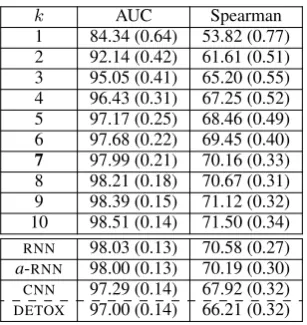
from random users, 4K comments from banned users).19 _{The decisions of 10 randomly chosen}

annotators (possibly different per comment) were used to construct the gold label of each comment. The gold labels were then compared to the deci-sions of the systems and the decideci-sions of an en-semble ofkother annotators,kranging from 1 to 10. Table3 shows the mean AUC and Spearman

scores, averaged over 25 runs of the experiment, along with standard errrors (in brackets). We con-clude that RNN anda-RNN are as good as an

en-semble of 7 human annotators;CNNis as good as

4 annotators;DETOXis as good as 4 inAUCand 3

annotators in Spearman correlation, which is con-sistent with the results of Wulczyn et al. (2017).

k AUC Spearman

1 84.34 (0.64) 53.82 (0.77) 2 92.14 (0.42) 61.61 (0.51) 3 95.05 (0.41) 65.20 (0.55) 4 96.43 (0.31) 67.25 (0.52) 5 97.17 (0.25) 68.46 (0.49) 6 97.68 (0.22) 69.45 (0.40) 7 97.99 (0.21) 70.16 (0.33) 8 98.21 (0.18) 70.67 (0.31) 9 98.39 (0.15) 71.12 (0.32) 10 98.51 (0.14) 71.50 (0.34) RNN 98.03 (0.13) 70.58 (0.27)

a-RNN 98.00 (0.13) 70.19 (0.30) CNN 97.29 (0.14) 67.92 (0.32) DETOX 97.00 (0.14) 66.21 (0.32)

Table 3: Comparing to an ensemble ofkhumans.

4.2 Snippet highlighting evaluation

To investigate if the attention scores of a-RNN

can highlight suspicious words, we focused onG -TEST-S-R, the only dataset with suspicious

snip-pets annotated by humans. We removed comments with no human-annotated snippets, leaving 841 comments (515 accepted, 326 rejected), a total of 40,572 tokens, of which 13,146 were inside a sus-picious snippet of at least one annotator. In each remaining comment, each token was assigned a

gold suspiciousnessscore, defined as the percent-age of annotators that included it in their snippets. We evaluated three methods that score each to-ken wt of a commentc for suspiciousness. The first one assigns to eachwtthe attention scoreat

19_{We used the protocol, code, and data of Wulczyn et al.}

Figure 7: Suspicious snippet highlighting results.

(Eq. 3) of a-RNN (trained on G-TRAIN-L). The

second method assigns to eachwtits precision, as computed byLIST(Section3.4). The third method

(RAND) assigns to eachwta random (uniform dis-tribution) score between 0 and 1. In the latter two methods, asoftmax is applied to the scores of all the tokens per comment, as ina-RNN. Figure6

shows three comments (fromW-ATT-TEST)

high-lighted bya-RNN; heat corresponds to attention.20

We computed Pearson and Spearman correla-tions between the gold suspiciousness scores and the scores of the three methods on the 40,572 to-kens. Figure 7 shows the correlations on com-ments that were accepted (left) and rejected (right) by the majority of moderators. In both cases,

a-RNN performs better than LIST and RAND by

both Pearson and Spearman correlations. The high Pearson correlations of a-RNN also show that its

attention scores are to a large extent linearly re-lated to the gold ones. By contrast,LISTperforms

reasonably well in terms of Spearman correlation, but much worse in terms of Pearson, indicating that its precision scores rank reasonably well the tokens from most to least suspicious ones, but are not linearly related to the gold scores.

5 Related work

Djuric et al. (2015) experimented with 952K man-ually moderated comments from Yahoo Finance, but their dataset is not publicly available. They convert each comment to a comment embedding using DOC2VEC (Le and Mikolov, 2014), which

is then fed to anLRclassifier. Nobata et al. (2016)

experimented with approx. 3.3M manually mod-erated comments from Yahoo Finance and News; their data are also not available.21 _{They used}

Vowpal Wabbit22 _{with character n-grams (n =}

3, . . . ,5) and word n-grams (n = 1,2), hand-crafted features (e.g., number of capitalized or black-listed words), features based on dependency

20_{In innocent comments,a-RNNspreads its attention to all} tokens, leading to quasi-uniform low color intensity.

21_{According to Nobata et al., their clean test dataset (2K} comments) would be made available, but it is currently not.

trees, averages of WORD2VEC embeddings, and DOC2VEC-like embeddings. Character n-grams

were the best, on their own outperforming Djuric et al. (2015). The best results, however, were ob-tained using all features. We use no hand-crafted features and parsers, making our methods more easily portable to other domains and languages.

Mehdad et al. (2016) train a (token or character-based)RNNlanguage model per class (accept,

re-ject), and use the probability ratio of the two mod-els to accept or reject user comments. Experi-ments on the dataset of Djuric et al. (2015), how-ever, showed that their method (RNNLMs)

per-formed worse than a combination of SVM and

Naive Bayes classifiers (NBSVM) that used

char-acter and tokenn-grams. AnLRclassifier

operat-ing on DOC2VEC-like comment embeddings (Le

and Mikolov, 2014) also performed worse than

NBSVM. To surpassNBSVM, Mehdad et al. used

anSVMto combine features from their three other

methods (RNNLMs,LRwithDOC2VEC,NBSVM).

Wulczyn et al. (2017) experimented with char-acter and wordn-grams. We included their dataset and moderation system (DETOX) in our

experi-ments. Waseem et al. (2016) used approx. 17K tweets annotated for hate speech. Their best re-sults were obtained using an LR classifier with

character n-grams (n = 1, . . . ,4), plus gender. Warner and Hirschberg (2012) aimed to detect anti-semitic speech, experimenting with 9K para-graphs and a linearSVM. Their features consider

windows of at most 5 tokens, examining the to-kens of each window, their order,POStags, Brown

clusters etc., following Yarowsky (1994).

Cheng et al. (2015) aimed to predict which users would be banned from on-line communities. Their best system used a random forest orLRclassifier,

with features examining readability, activity (e.g., number of posts daily), community and moderator reactions (e.g., up-votes, number of deleted posts). Sood et al. (2012a;2012b) experimented with 6.5K comments from Yahoo Buzz, moderated via crowdsourcing. They showed that a linear SVM,

representing each comment as a bag of word bi-grams and stems, performs better than word lists. Their best results were obtained by combining the

SVMwith a word list and edit distance.

Yin et al. (2009) used posts from chat rooms and discussion fora (<15K posts in total) to train an SVM to detect online harassment. They used TF-IDF, sentiment, and context features (e.g.,

sim-ilarity to other posts in a thread). Our methods might also benefit by considering threads, rather than individual comments. Yin at al. point out that unlike other abusive content, spam in comments or dicsussion fora (Mishne et al.,2005;Niu et al.,

2007) is off-topic and serves a commercial pur-pose. Spam is unlikely in Wikipedia discussions and not an issue in the Gazzetta dataset (Fig.2).

For a more extensive discussion of related work, consult Pavlopoulos et al. (2017).

6 Conclusions

We experimented with a new publicly available dataset of 1.6M moderated user comments from a Greek sports news portal and an existing dataset of 115K English Wikipedia talk page comments. We showed that a GRU RNN operating on word

embeddings outpeforms the previous state of the art, which used anLRorMLPclassifier with

char-acter or word n-gram features, also outperform-ing a vanillaCNNoperating on word embeddings,

and a baseline that uses an automatically con-structed word list with precision scores. A novel, deep, classification-specific attention mechanism improves further the overall results of the RNN,

and can also highlight suspicious words for free, without including highlighted words in the train-ing data. We considered both fully automatic and semi-automatic moderation, along with threshold tuning and evaluation measures for both.

We plan to consider user-specific information (e.g., ratio of comments rejected in the past) (Cheng et al., 2015; Waseem and Hovy, 2016) and explore character-levelRNNs orCNNs (Zhang

et al., 2015), e.g., as a first layer to produce em-beddings of unknown words from characters (dos Santos and Zadrozny, 2014; Ling et al., 2015), which would then be passed on to our current methods that operate on word embeddings.

Acknowledgments

This work was funded by Google’s Digital News Initiative (projectML2P, contract 362826).23 We

are grateful to Gazzetta for the data they pro-vided. We also thank Gazzetta’s moderators for their feedback, insights, and advice.

References

Dzmitry Bahdanau, Kyunghyun Cho, and Yoshua Ben-gio. 2015. Neural machine translation by jointly learning to align and translate. In Proceedings of the 3rd International Conference on Learning Rep-resentations. San Diego, CA, USA.

Justin Cheng, Cristian Danescu-Niculescu-Mizil, and Jure Leskovec. 2015. Antisocial behavior in online discussion communities. InProceedings of the 9th International AAAI Conference on Web and Social Media. Oxford University, England, pages 61–70. Kyunghyun Cho, Bart van Merrienboer, Caglar

Gul-cehre, Dzmitry Bahdanau, Fethi Bougares, Holger Schwenk, and Yoshua Bengio. 2014. Learning phrase representations using RNN encoder–decoder for statistical machine translation. InProceedings of the 2014 Conference on Empirical Methods in Natu-ral Language Processing. Doha, Qatar, pages 1724– 1734.

Jacob Cohen. 1960. A coefficient of agreement for nominal scales. Educational and Psychological Measurement20(1):37–46.

Nemanja Djuric, Jing Zhou, Robin Morris, Mihajlo Gr-bovic, Vladan Radosavljevic, and Narayan Bhamidi-pati. 2015. Hate speech detection with comment embeddings. In Proceedings of the 24th Interna-tional Conference on World Wide Web. Florence, Italy, pages 29–30.

C´ıcero Nogueira dos Santos and Bianca Zadrozny. 2014. Learning character-level representations for part-of-speech tagging. In Proceedings of the 31st International Conference on Machine Learn-ing. Beijing, China, pages 1818–1826.

Xavier Glorot and Yoshua Bengio. 2010. Understand-ing the difficulty of trainUnderstand-ing deep feedforward neural networks. InProceedings of the International Con-ference on Artificial Intelligence and Statistics. Sar-dinia, Italy, pages 249–256.

Yoav Goldberg. 2016. A primer on neural network models for natural language processing. Journal of Artificial Intelligence Research57:345–420. Yoav Goldberg. 2017. Neural Network Methods in

Natural Language Processing. Morgan and Clay-pool Publishers.

Ian Goodfellow, Yoshua Bengio, and Aaron Courville. 2016.Deep Learning. MIT Press.

Geoffrey E. Hinton, Nitish Srivastava, Alex Krizhevsky, Ilya Sutskever, and Ruslan Salakhut-dinov. 2012. Improving neural networks by preventing co-adaptation of feature detectors. CoRR

abs/1207.0580.

Yoon Kim. 2014. Convolutional neural networks for sentence classification. InProceedings of the 2014 Conference on Empirical Methods in Natural Lan-guage Processing. Doha, Qatar, pages 1746–1751.

Diederik P. Kingma and Jimmy Ba. 2015. Adam: A method for stochastic optimization. In Proceed-ings of the 3rd International Conference on Learn-ing Representations. San Diego, CA, USA.

Klaus Krippendorff. 2004. Content Analysis: An In-troduction to Its Methodology (2nd edition). Sage Publications.

Quoc V. Le and Tomas Mikolov. 2014. Distributed representations of sentences and documents. In

Proceedings of the 31st International Conference on Machine Learning. Beijing, China, pages 1188– 1196.

Wang Ling, Chris Dyer, Alan W. Black, Isabel Tran-coso, Ramon Fermandez, Silvio Amir, Lu´ıs Marujo, and Tiago Lu´ıs. 2015. Finding function in form: Compositional character models for open vocabu-lary word representation. InProceedings of the Con-ference on Empirical Methods in Natural Language Processing. Lisbon, Portugal, pages 1520–1530. Thang Luong, Hieu Pham, and Christopher D.

Man-ning. 2015. Effective approaches to attention-based neural machine translation. In Proceedings of the 2015 Conference on Empirical Methods in Natu-ral Language Processing. Lisbon, Portugal, pages 1412–1421.

Yashar Mehdad and Joel Tetreault. 2016. Do charac-ters abuse more than words? InProceedings of the 17th Annual Meeting of the Special Interest Group on Discourse and Dialogue. Los Angeles, CA, pages 299–303.

Tomas Mikolov, Kai Chen, Greg Corrado, and Jeffrey Dean. 2013a. Efficient estimation of word represen-tations in vector space. InProceedings of Workshop at International Conference on Learning Represen-tations. Scottsdale, AZ, USA.

Tomas Mikolov, Wen-tau Yih, and Geoffrey Zweig. 2013b. Linguistic regularities in continuous space word representations. InProceedings of the 2013 Conference of the North American Chapter of the Association for Computational Linguistics: Human Language Technologies. Atlanta, GA, pages 746– 751.

Gilad Mishne, David Carmel, and Ronny Lempel. 2005. Blocking blog spam with language model dis-agreement. InProceedings of the 1st International Workshop on Adversarial Information Retrieval on the Web. Chiba, Japan.

Volodymyr Mnih, Nicolas Heess, Alex Graves, et al. 2014. Recurrent models of visual attention. In Ad-vances in Neural Information Processing Systems. Montreal, Canada, pages 2204–2212.

Yuan Niu, Yi-Min Wang, Hao Chen, Ming Ma, and Francis Hsu. 2007. A quantitative study of fo-rum spamming using context-based analysis. In

Chikashi Nobata, Joel Tetreault, Achint Thomas, Yashar Mehdad, and Yi Chang. 2016. Abusive lan-guage detection in online user content. In Proceed-ings of the 25th International Conference on World Wide Web. Montreal, Canada, pages 145–153. John Pavlopoulos, Prodromos Malakasiotis, and Ion

Androutsopoulos. 2017. Deep learning for user comment moderation. InProceedings of the 1st ACL Workshop on Abusive Language Online. Vancouver, Canada.

Jeffrey Pennington, Richard Socher, and Christopher Manning. 2014. GloVe: Global vectors for word representation. In Proceedings of the 2014 Con-ference on Empirical Methods in Natural Language Processing. Doha, Qatar, pages 1532–1543. Mike Schuster and Kuldip K Paliwal. 1997.

Bidirec-tional recurrent neural networks. IEEE Transacions of Signal Processing45(11):2673–2681.

Sara Sood, Judd Antin, and Elizabeth F. Churchill. 2012a. Profanity use in online communities. In Pro-ceedings of the SIGCHI Conference on Human Fac-tors in Computing Systems. Austin, TX, USA, pages 1481–1490.

Sara Sood, Judd Antin, and Elizabeth F. Churchill. 2012b. Using crowdsourcing to improve profanity detection. InAAAI Spring Symposium: Wisdom of the Crowd. Stanford, CA, USA, pages 69–74. Ilya Sutskever, Oriol Vinyals, and Quoc V. Le. 2014.

Sequence to sequence learning with neural net-works. InAdvances in Neural Information Process-ing Systems. Montreal, Canada, pages 3104–3112. William Warner and Julia Hirschberg. 2012. Detecting

hate speech on the World Wide Web. In Proceed-ings of the 2nd Workshop on Language in Social Me-dia. Montreal, Canada, pages 19–26.

Zeerak Waseem and Dirk Hovy. 2016. Hateful sym-bols or hateful people? Predictive features for hate speech detection on Twitter. In Proceedings of the NAACL Student Research Workshop. San Diego, CA, USA, pages 88–93.

Ellery Wulczyn, Nithum Thain, and Lucas Dixon. 2017. Ex machina: Personal attacks seen at scale. InProceedings of the 26th International Conference on World Wide Web. Perth, Australia, pages 1391– 1399.

Kelvin Xu, Jimmy Ba, Ryan Kiros, Kyunghyun Cho, Aaron Courville, Ruslan Salakhutdinov, Richard Zemel, and Yoshua Bengio. 2015. Show, attend and tell: Neural image caption generation with visual at-tention. InICML. Lille, France, pages 2048–2057. Zichao Yang, Diyi Yang, Chris Dyer, Xiaodong He,

Alex Smola, and Eduard Hovy. 2016. Hierarchi-cal attention networks for document classification. InProceedings of the 2016 Conference of the North

American Chapter of the Association for Computa-tional Linguistics: Human Language Technologies. San Diego, CA, USA, pages 1480–1489.

David Yarowsky. 1994. Decision lists for lexical ambi-guity resolution: Application to accent restoration in Spanish and French. InProceedings of the 32nd An-nual Meeting of the Association for Computational Linguistics. Las Cruces, NM, USA, pages 88–95. Dawei Yin, Zhenzhen Xue, Liangjie Hong, Brian D

Davison, April Kontostathis, and Lynne Edwards. 2009. Detection of harassment on Web 2.0. In Pro-ceedings of the WWW workshop on Content Analysis in the Web 2.0. Madrid, Spain.

Xiang Zhang, Junbo Zhao, and Yann LeCun. 2015. Character-level convolutional networks for text clas-sification. InProceedings of the 28th International Conference on Neural Information Processing Sys-tems. Montreal, Canada, pages 649–657.

Ye Zhang and Byron C. Wallace. 2015. A sensitiv-ity analysis of (and practitioners’ guide to) convo-lutional neural networks for sentence classification.