Left-to-Right Tree-to-String Decoding with Prediction
Yang Feng† Yang Liu‡ Qun Liu⋆ Trevor Cohn†
†Department of Computer Science
The University of Sheffield, Sheffield, UK
{y.feng, t.cohn}@sheffield.ac.uk
‡State Key Laboratory on Intelligent Technology and Systems
Tsinghua National Laboratory for Information Science and Technology Department of Computer Sci. and Tech., Tsinghua University, Beijing, China
⋆Key Laboratory of Intelligent Information Processing
Institute of Computing Technology Chinese Academy of Sciences, Beijing, China
Abstract
Decoding algorithms for syntax based ma-chine translation suffer from high compu-tational complexity, a consequence of in-tersecting a language model with a con-text free grammar. Left-to-right decoding, which generates the target string in order, can improve decoding efficiency by simpli-fying the language model evaluation. This paper presents a novel left to right decod-ing algorithm for tree-to-strdecod-ing translation, us-ing a bottom-up parsus-ing strategy and dynamic future cost estimation for each partial trans-lation. Our method outperforms previously published tree-to-string decoders, including a competing left-to-right method.
1 Introduction
In recent years there has been rapid progress in the development of tree-to-string models for statistical machine translation. These models use the syntac-tic parse tree of the source language to inform its translation, which allows the models to capture con-sistent syntactic transformations between the source and target languages, e.g., from subject-verb-object to subject-object-verb word orderings. Decoding al-gorithms for grammar-based translation seek to find the best string in the intersection between a weighted context free grammar (the translation mode, given a source string/tree) and a weighted finite state accep-tor (an n-gram language model). This intersection
is problematic, as it results in an intractably large grammar, and makes exact search impossible.
Most researchers have resorted to approximate search, typically beam search (Chiang, 2007). The decoder parses the source sentence, recording the target translations for each span.1 As the partial translation hypothesis grows, its component ngrams are scored and the hypothesis score is updated. This decoding method though is inefficient as it requires recording the language model context (n−1words) on the left and right edges of each chart cell. These contexts allow for boundary ngrams to be evaluated when the cell is used in another grammar produc-tion. In contrast, if the target string is generated in left-to-right order, then only one language model context is required, and the problem of language model evaluation is vastly simplified.
In this paper, we develop a novel method of left-to-right decoding for tree-to-string translation using a shift-reduce parsing strategy. A central issue in any decoding algorithm is the technique used for pruning the search space. Our left-to-right decod-ing algorithm groups hypotheses, which cover the same number of source words, into a bin. Pruning requires the evaluation of different hypotheses in the same bin, and elimating the least promising options. As each hypotheses may cover different sets of tree
1The process is analogous for tree-to-string models, except
that only rules and spans matching those in the source trees are considered. Typically nodes are visited according to a post-order traversal.
nodes, it is necessary to consider the cost of uncov-ered nodes, i.e., thefuture cost. We show that a good future cost estimate is essential for accurate and effi-cient search, leading to high quality translation out-put.
Other researchers have also considered the left-to-right decoding algorithm for tree-to-string mod-els. Huang and Mi (2010) developed an Earley-style parsing algorithm (Earley, 1970). In their ap-proach, hypotheses covering the same number of tree nodes were binned together. Their method uses a top-down depth-first search, with a mechanism for early elimation of some rules which lead to dead-ends in the search. Huang and Mi (2010)’s method was shown to outperform the traditional post-order-traversal decoding algorithm, considering fewer hy-potheses and thus decoding much faster at the same level of performance. However their algorithm used a very rough estimate of future cost, resulting in more search errors than our approach.
Our experiments show that compared with the Earley-style left-to-right decoding (Huang and Mi, 2010) and the traditional post-order-traversal de-coding (Liu et al., 2006) algorithms, our algorithm achieves a significant improvement on search capac-ity and better translation performance at the same level of speed.
2 Background
A typical tree-to-string system (Liu et al., 2006; Huang et al., 2006) searches through a 1-best source parse tree for the best derivation. It transduces the source tree into a target-language string using a Syn-chronous Tree Substitution Grammar (STSG). The grammar rules are extracted from bilingual word alignments using the GHKM algorithm (Galley et al., 2004).
We will briefly review the traditional decoding al-gorithm (Liu et al., 2006) and the Earley-style top-down decoding algorithm (Huang and Mi, 2010) for the tree-to-string model.
2.1 Traditional Decoding
The traditional decoding algorithm processes source tree nodes one by one according to a post-order traversal. For each node, it applies matched STSG rules by substituting each non-terminal with its
cor-in theory beam search traditional O(nc˙|V|4(g−1)) O(ncb2) top-down O(c(cr)d|V|g−1) O(ncb) bottom-up O((cr)d|V|g−1) O(nub)
Table 1: Time complexity of different algorithms. tra-ditional: Liu et al. (2006), top-down : Huang and Mi (2010). n is the source sentence length, b is the beam width, c is the number of rules used for each node, V is the target word vocabulary,g is the order of the lan-guage model,dis the depth of the source parse tree,uis the number of viable prefixes for each node andris the maximum arity of each rule.
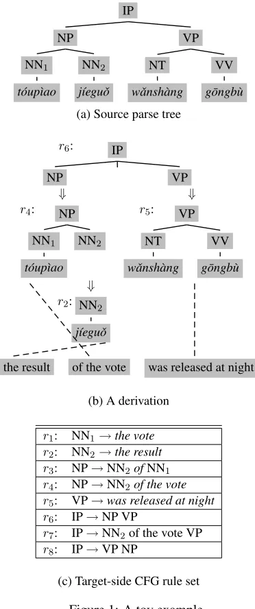
responding translation. For the derivation in Figure 1 (b), the traditional algorithm applies r2 at node
NN2
r2 : NN2(jieguo)→the result,
to obtain “the result” as the translation of NN2. Next
it appliesr4at node NP,
r4: NP ( NN1(toupiao), x1:NN2 )
→x1of the vote
and replaces NN2 with its translation “the result”,
then it gets the translation of NP as “the result of the vote”.
This algorithm needs to contain boundary words at both left and right extremities of the target string for the purpose of LM evaluation, which leads to a high time complexity. The time complexity in the-ory and with beam search (Huang and Mi, 2010) is shown in Table 1.
2.2 Earley-style Top-down Decoding
The Earley-style decoding algorithm performs a top-down depth-first parsing and generates the target translation left to right. It applies Context-Free Grammar (CFG) rules and employs three actions:
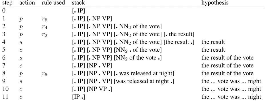
predict, scan and complete (Section 3.1 describes how to convert STSG rules into CFG rules). We can simulate its translation process using a stack with a dotindicating which symbol to process next. For the derivation in Figure 1(b) and CFG rules in Fig-ure 1(c), FigFig-ure 2 illustrates the whole translation process.
3 Bottom-Up Left-to-Right Decoding
We propose a novel method of left-to-right decoding for tree-to-string translation using a bottom-up pars-ing strategy. We useviable prefixes(Aho and John-son, 1974) to indicate all possible target strings the translations of each node should starts with. There-fore, given a tree node to expand, our algorithm can drop immediately to target terminals no matter whether there is agapor not. We say that there is a gap between two symbols in a derivation when there are many rules separating them, e.g. IP→r6 ... →r4
NN2. For the derivation in Figure 1(b), our
algo-rithm starts from the root node IP and applies r2
first although there is a gap between IP and NN2.
Then it appliesr4,r5andr6in sequence to generate
the translation “the result of the vote was released at night”. Our algorithm takes the gap as a black-box and does not need to fix which partial deriva-tion should be used for the gap at the moment. So it can get target strings as soon as possible and thereby perform more accurate pruning. A valid derivation is generated only when the source tree is completely matched by rules.
Our bottom-up decoding algorithm involves the following steps:
1. Match STSG rules against the source tree.
2. Convert STSG rules to CFG rules.
3. Collect the viable prefix set for each node in a post-order transversal.
4. Search bottom-up for the best derivation.
3.1 From STSG to CFG
After rule matching, each tree node has its applica-ble STSG rule set. Given a matched STSG rule, our decoding algorithm only needs to consider the tree node the rule can be applied to and the target side, so we follow Huang and Mi (2010) to convert STSG rules to CFG rules. For example, an STSG rule
NP ( NN1(toupiao), x1:NN2)→x1of the vote
can be converted to a CFG rule
NP→NN2 of the vote
The target non-terminals are replaced with corre-sponding source non-terminals. Figure 1 (c) shows all converted CFG rules for the toy example. Note
IP
NP
NN1
t´oup`ıao
NN2
j´ıeguˇo
VP
NT
wˇansh`ang
VV
g¯ongb`u
(a) Source parse tree
r6: IP
NP VP
⇓ ⇓
r4: NP
NN1
t´oup`ıao NN2
r5: VP
NT
wˇansh`ang
VV
g¯ongb`u
⇓
r2: NN2
j´ıeguˇo
the result of the vote was released at night
(b) A derivation
r1: NN1→the vote
r2: NN2→the result
r3: NP→NN2ofNN1
r4: NP→NN2of the vote
r5: VP→was released at night
r6: IP→NP VP
r7: IP→NN2of the vote VP
r8: IP→VP NP
[image:3.612.326.512.54.498.2](c) Target-side CFG rule set
Figure 1: A toy example.
that different STSG rules might be converted to the same CFG rule despite having different source tree structures.
3.2 Viable Prefix
During decoding, how do we decide which rules should be used next given a partial derivation, es-pecially when there is a gap? A key observation is that some rules should be excluded. For example, any derivation for Figure 1(a) will never begin with
r1as there is no translation starting with “the vote”.
NN1: {the vote} NN2: {the result}
NT: ∅ VV: ∅
NP: {the result}
[image:4.612.89.283.61.130.2]VP: {was released at night} IP: {the result, was released at night}
Table 2: The Viable prefix sets for Figure 1 (c)
according to r1, the starting terminal string of the
translation for NN1 is “the vote”. According tor2,
the starting terminal string for NN2 is “the result”.
According to r3, the starting terminal string of NP
must include that of NN2. Table 2 lists the starting
terminal strings of all nodes in Figure 1(a). As the translations of node IP should begin with either “the result” or “was released at night”, the first rule must be eitherr2 orr5. Therefore, r1 will never be used
as the first rule in any derivation.
We refer to starting terminal strings of a node as a viable prefixes, a term borrowed from LR pars-ing (Aho and Johnson, 1974). Viable prefixes are used to decide which rule should be used to ensure efficient left-to-right target generation. Formally, as-sume thatVN denotes the set of non-terminals (i.e., source tree node labels), VT denotes the set of ter-minals (i.e., target words),v1, v2 ∈ VN,w ∈ VT ,
π∈ {VT ∪ VN}∗, we say thatwis a viable prefix of
v1if and only if:
• v1 →w, or
• v1 →wv2π, or
• v1 →v2π, andwis a viable prefix ofv2.
Note that we bundle all successive terminals in one symbol.
3.3 Shift-Reduce Parsing
We use a shift-reduce algorithm to search for the best deviation. The algorithm maintains a stack of dotted rules (Earley, 1970). Given the source tree in Figure 1(a), the stack is initialized with a dotted rule for the root node IP:
[IP].
Then, the algorithm selects one viable prefix of IP and appends it to the stack with the dot at the begin-ning (predict):
[IP] [the result]2.
Then, ascanaction is performed to produce a partial translation “the result”:
[IP] [the result].
Next, the algorithm searches for the CFG rules start-ing with “the result” and getsr2. Then, it pops the
rightmost dotted rule and append the left-hand side (LHS) ofr2to the stack (complete):
[IP] [NN2].
Next, the algorithm chooses r4 whose right-hand
side “NN2 of the vote” matches the rightmost dot-ted rule in the stack3andgrowsthe rightmost dotted rule:
[IP] [NN2of the vote].
Figure 3 shows the whole process of derivation generation.
Formally, we define four actions on the rightmost rule in the stack:
• Predict. If the symbol after the dot in the right-most dotted rule is a non-terminalv, this action chooses a viable prefixwofv and generates a new dotted rule forwwith the dot at the begin-ning. For example:
[IP]predict−→ [IP] [the result]
• Scan. If the symbol after the dot in the right-most dotted rule is a terminal stringw, this ac-tion advances the dot to update the current par-tial translation. For example:
[IP] [the result]scan−→[IP] [the result]
• Complete. If the rightmost dotted rule ends with a dot and it happens to be the right-hand side of a rule, then this action removes the right-most dotted rule. Besides, if the symbol after the dot in the new rightmost rule corre-sponds to the same tree node as the LHS non-terminal of the rule, this action advance the dot. For example,
[IP] [NPVP] [was released at night] complete
−→ [IP] [NP VP]
2
There are another option: “was released at night”
3
step action rule used stack hypothesis
0 [IP]
1 p r6 [IP] [NP VP]
2 p r4 [IP] [NP VP] [NN2of the vote]
3 p r2 [IP] [NP VP] [NN2of the vote] [the result]
4 s [IP] [NP VP] [NN2of the vote] [the result] the result
5 c [IP] [NP VP] [NN2 of the vote] the result
6 s [IP] [NP VP] [NN2 of the vote] the result of the vote
7 c [IP] [NPVP] the result of the vote
8 p r5 [IP] [NPVP] [was released at night] the result of the vote
9 s [IP] [NPVP] [was released at night] the ... vote was ... night
10 c [IP] [NP VP] the ... vote was ... night
[image:5.612.74.543.64.242.2]11 c [IP] the ... vote was ... night
Figure 2: Simulation of top-down translation process for the derivation in Figure 1(b). Actions:p, predict;s, scan;c, complete. “the ... vote” and “was ... released” are the abbreviated form of “the result of the vote” and “was released at night”, respectively.
step action rule used stack number hypothesis
0 [IP] 0
1 p [IP] [the result] 0
2 s [IP] [the result] 1 the result
3 c r2 [IP] [NN2] 1 the result
4 g r4orr7 [IP] [NN2of the vote] 1 the result
5 s [IP] [NN2of the vote] 2 the result of the vote
6 c r4 [IP] [NP] 2 the result of the vote
7 g r6 [IP] [NPVP] 2 the result of the vote
8 p [IP] [NPVP] [was released at night] 2 the result of the vote 9 s [IP] [NPVP] [was released at night] 4 the ... vote was ... night
10 c r5 [IP] [NP VP] 4 the ... vote was ... night
11 c r6 [IP] 4 the ... vote was ... night
Figure 3: Simulation of bottom-up translation process for the derivation in Figure 1(b). Actions:p, predict;s, scan;c, complete;g, grow. The column ofnumbergives the number of source words the hypothesis covers.
If the string cannot rewrite on the frontier non-terminal, then we add the LHS to the stack with the dot after it. For example:
[IP] [the result]complete−→ [IP] [NN2]
• Grow. If the right-most dotted rule ends with a dot and it happens to be the starting part of a CFG rule, this action appends one symbol of the remainder of that rule to the stack4. For example:
4We bundle the successive terminals in one rule into a
sym-bol
[IP] [NN2]
grow
−→[IP] [NN2of the vote]
From the above definition, we can find that there may be an ambiguity about whether to use a com-plete action or a grow action. Similarly, predict ac-tions must select a viable prefix form the set for a node. For example in step 5, although we select to perform complete with r4 in the example, r7 is
applicable, too. In our implementation, if bothr4
andr7are applicable, we apply them both to
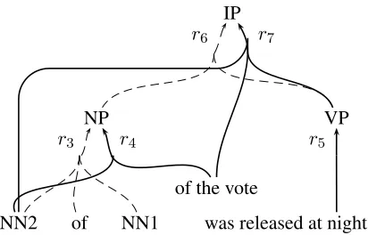
IP
NP
NN2 of NN1
of the vote
VP
was released at night
r7
r4 r5
r6
[image:6.612.83.289.59.191.2]r3
Figure 4: The translation forest composed of applicable CFG rules for the partial derivation of step 3 in Figure 3.
3.4 Future Cost
Partial derivations covering different tree nodes may be grouped in the same bin for beam pruning5. In order to perform more accurate pruning, we take into considerationfuture cost, the cost of the uncovered part. Themeritof a derivation is thecovered cost
(the cost of the covered part) plus the future cost. We borrow ideas from the Inside-Outside algorithm (Charniak and Johnson, 2005; Huang, 2008; Mi et al., 2008) to compute the merit. In our algorithm, the merit of a derivation is just the Viterbi inside cost
β of the root node calculated with the derivations continuing from the current derivation.
Given a partial derivation, we calculate its future cost by searching through the translation forest de-fined by all applicable CFG rules. Figure 4 shows the translation forest for the derivation of step 3. We calculate the future cost for each node as follows: given a nodev, we define its cost functionf(v)as
f(v) =
1 vis completed
lm(v) vis a terminal string maxr∈Rvf(r)
∏
π∈rhs(r)f(π)otherwise
whereVN is the non-terminal set,VT is the terminal set,v, π ∈VN∪VT+,Rv is the set of currently ap-plicable rules forv,rhs(r)is the right-hand symbol set ofr,lmis the local language model probability,
f(r) is calculated using a linear model whose fea-tures are bidirectional translation probabilities and lexical probabilities of r. For the translation forest in Figure 4, if we calculate the future cost of NP with
5
Section 3.7 will describe the binning scheme
r4, then
f(N P) = f(r4)·f(N N2)·lm(of the vote)
= f(r4)·1·lm(of the vote)
Note that we calculatelm(of the vote) locally and do not take “the result” derived from NN2 as the
con-text. The lm probability of “the result” has been in-cluded in the covered cost.
As a partial derivation grows, some CFG rules will conflict with the derivation (i.e. inapplicable) and the translation forest will change accordingly. For example, when we reach step 5 from step 3 (see Figure 4 for its translation forest), r3 is
inapplica-ble and thereby should be ruled out. Then the nodes on the path from the last covered node (it is “of the vote” in step 5) to the root node should update their future cost, as they may employ r3 to produce the
future cost. In step 5, NP and IP should be updated. In this sense, we say that the future cost is dynamic.
3.5 Comparison with Top-Down Decoding
In order to generate the translation “the result” based on the derivation in Figure 1(b), Huang and Mi’s top-down algorithm needs to specify which rules to apply starting from the root node until it yields “the result”. In this derivation, ruler6is applied to IP,r4
to NP,r2 toN N2. That is to say, it needs to
repre-sent the partial derivation from IP to NN2explicitly.
This can be a problem when combined with beam pruning. If the beam size is small, it may discard the intermediate hypotheses and thus never consider the string. In our example with a beam of 1, we must select a rule for IP amongr6,r7andr8although we
do not get any information for NP and VP.
3.6 Time Complexity
Assume the depth of the source tree isd, the max-imum number of matched rules for each node isc, the maximum arity of each rule is r, the language model order isgand the target-language vocabulary is V, then the time complexity of our algorithm is
O((cr)d|V|g−1). Analysis is as follows:
Our algorithm expands partial paths with termi-nal strings to generate new hypotheses, so the time complexity depends on the number of partial paths used. We split a path which is from the root node to a leaf node with a node on it (called the end node) and get the segment from the root node to the end node as a partial path, so the length of the partial path is not definite with a maximum ofd. If the length is
d′(d′ ≤d), then the number of partial paths is(cr)d′. Besides, we use the rightestg−1 words to signa-ture each partial path, so we can get (cr)d′|V|g−1
states. For each state, the number of viable prefixes produced by predict operation iscd−d′, so the total time complexity is f = O((cr)d′|V|g−1cd−d′) =
O(cdrd′|V|g−1) =O((cr)d|V|g−1).
3.7 Beam Search
To make decoding tractable, we employ beam search (Koehn, 2004) and choose “binning” as follows: hy-potheses covering the same number of source words are grouped in a bin. When expanding a hypothe-sis in a beam (bin), we take series of actions until new terminals are appended to the hypothesis, then add the new hypothesis to the corresponding beam. Figure 3 shows the number of source words each hy-pothesis covers.
Among the actions, only the scan action changes the number of source words each hypothesis cov-ers. Although the complete action does not change source word number, it changes the covered cost of hypotheses. So in our implementation, we take scan and complete as “closure” actions. That is to say, once there are some complete actions after a scan ac-tion, we finish all the compete actions until the next action is grow. The predict and grow actions decide which rules can be used to expand hypotheses next, so we update the applicable rule set during these two actions.
Given a source sentence withnwords, we main-tainnbeams, and let each beam holdbhypotheses
at most. Besides, we prune viable prefixes of each node up tou, so each hypothesis can expand tou
new hypotheses at most, so the time complexity of beam search isO(nub).
4 Related Work
Watanabe et al. (2006) present a novel Earley-style top-down decoding algorithm for hierarchical phrase-based model (Chiang, 2005). Their frame-work extracts Greibach Normal Form rules only, which always has at least one terminal on the left of each rule, and discards other rules.
Dyer and Resnik (2010) describe a translation model that combines the merits of syntax-based models and phrase-based models. Their decoder works in two passes: for first pass, the decoder col-lects a context-free forest and performs tree-based source reordering without a LM. For the second pass, the decoder adds a LM and performs bottom-up CKY decoding.
Feng et al. (2010) proposed a shift-reduce algo-rithm to add BTG constraints to phrase-based mod-els. This algorithm constructs a BTG tree in a reduce-eager manner while the algorithm in this pa-per searches for a best derivation which must be de-rived from the source tree.
Galley and Manning (2008) use the shift-reduce algorithm to conduct hierarchical phrase reordering so as to capture long-distance reordering. This al-gorithm shows good performance on phrase-based models, but can not be applied to syntax-based mod-els directly.
5 Experiments
5.1 Data Setup
We used the FBIS corpus consisting of about 250K Chinese-English sentence pairs as the training set. We aligned the sentence pairs using the GIZA++ toolkit (Och and Ney, 2003) and extracted tree-to-string rules according to the GHKM algorithm (Gal-ley et al., 2004). We used the SRILM toolkit (Stol-cke, 2002) to train a 4-gram language model on the Xinhua portion of the GIGAWORD corpus.
We used the 2002 NIST MT Chinese-English test set (571 sentences) as the development set and the 2005 NIST MT Chinese-English test set (1082 sen-tences) as the test set. We evaluated translation qual-ity using BLEU-metric (Papineni et al., 2002) with case-insensitiven-gram matching up ton = 4. We used the standard minimum error rate training (Och, 2003) to tune feature weights to maximize BLEU score on the development set.
5.2 Performance Comparison
Our bottom-up left-to-right decoder employs the same features as the traditional decoder: rule proba-bility, lexical probaproba-bility, language model probabil-ity, rule count and word count. In order to compare them fairly, we used the same beam size which is20 and employed cube pruning technique (Huang and Chiang, 2005).
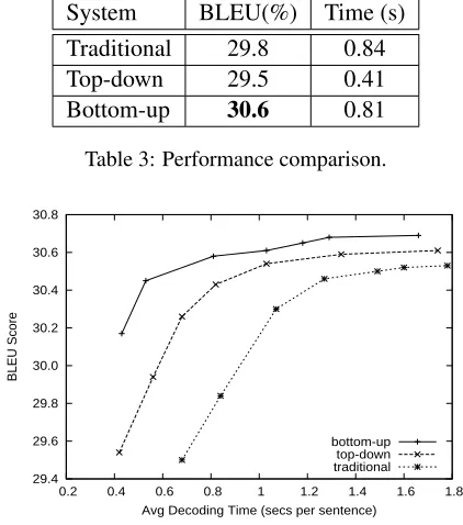
We show the results in Table 3. From the re-sults, we can see that the bottom-up decoder out-performs top-down decoder and traditional decoder by 1.1 and 0.8 BLEU points respectively and the improvements are statistically significant using the
sign-test of Collins et al. (2005) (p < 0.01). The improvement may result from dynamically search-ing for a whole derivation which leads to more ac-curate estimation of a partial derivation. The addi-tional time consumption of the bottom-up decoder against the top-down decoder comes from dynamic future cost computation.
Next we compare decoding speed versus transla-tion quality using various beam sizes. The results are shown in Figure 5. We can see that our bottom-up decoder can produce better BLEU score at the same decoding speed. At small beams (decoding time around 0.5 second), the improvement of trans-lation quality is much bigger.
System BLEU(%) Time (s)
Traditional 29.8 0.84
Top-down 29.5 0.41
[image:8.612.319.530.62.301.2]Bottom-up 30.6 0.81
Table 3: Performance comparison.
29.4 29.6 29.8 30.0 30.2 30.4 30.6 30.8
0.2 0.4 0.6 0.8 1 1.2 1.4 1.6 1.8
BLEU Score
Avg Decoding Time (secs per sentence) bottom-up
top-down traditional
Figure 5: BLEU score against decoding time with various beam size.
5.3 Search Capacity Comparison
We also compare the search capacity of the bottom-up decoder and the traditional decoder. We do this in the following way: we let both decoders use the same weights tuned on the traditional decoder, then we compare their translation scores of the same test sentence.
From the results in Table 4, we can see that for many test sentences, the bottom-up decoder finds target translations with higher score, which have been ruled out by the traditional decoder. This may result from more accurate pruning method. Yet for some sentences, the traditional decoder can attain higher translation score. The reason may be that the traditional decoder can hold more than two nonter-minals when cube pruning, while the bottom-up de-coder always performs dual-arity pruning.
statis-28.0 29.0 30.0 31.0 32.0 33.0 34.0 35.0
10 20 30 40
BLEU Score
Beam Size
[image:9.612.80.290.62.205.2]bottom-up traditional
Figure 6: BLEU score with various beam sizes on the sub test set consisting of sentences on which the bottom-up decoder gets higher translation score than the traditional decoder does.
b > = <
10 728 67% 347 32% 7 1%
20 657 61% 412 38% 13 1%
30 615 57% 446 41% 21 2%
40 526 49% 523 48% 33 3%
[image:9.612.83.290.275.361.2]50 315 29% 705 65% 62 6%
Table 4: Search capacity comparison. The first column is beam size, the following three columns denote the num-ber of test sentences, on which the translation scores of the bottom-up decoder are greater, equal to, lower than that of the traditional decoder.
System BLEU(%) Time (s)
with 30.6 0.81
without 28.8 0.39
Table 5: Influence of future cost. The results of the bottom-up decoder with and without future cost are given in the second and three rows, respectively.
tical distribution of hypotheses well. In addition, the weights are tuned on the traditional decoder, not on the bottom-up decoder. The bottom-up decoder can perform better with weights tuned by itself.
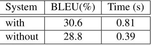
5.4 Influence of Future Cost
Next, we will show the impact of future cost via ex-periments. We give the results of the bottom-up de-coder with and without future cost in Table 5. From the result, we can conclude that future cost plays a significant role in decoding. If the bottom-up de-coder does not employ future cost, its performance
will be influenced dramatically. Furthermore, cal-culating dynamic future cost is time consuming. If the bottom-up decoder does not use future cost, it decodes faster than the top-down decoder. This is because the top-down decoder has|T|beams, while the bottom-up decoder hasnbeams, whereT is the source parse tree and nis the length of the source sentence.
6 Conclusions
In this paper, we describe a bottom-up left-to-right decoding algorithm for tree-to-string model. With the help of viable prefixes, the algorithm generates a translation by constructing a target-side CFG tree according to a post-order traversal. In addition, it takes into consideration a dynamic future cost to es-timate hypotheses.
On the 2005 NIST Chinese-English MT transla-tion test set, our decoder outperforms the top-down decoder and the traditional decoder by 1.1 and 0.8 BLEU points respectively and shows more powerful search ability. Experiments also prove that future cost is important for more accurate pruning.
7 Acknowledgements
We would like to thank Haitao Mi and Douwe Gelling for their feedback, and anonymous review-ers for their valuable comments and suggestions. This work was supported in part by EPSRC grant EP/I034750/1 and in part by High Technology R&D Program Project No. 2011AA01A207.
References
A. V. Aho and S. C. Johnson. 1974. Lr parsing. Com-puting Surveys, 6:99–124.
Eugene Charniak and Mark Johnson. 2005. Coarse-to-fine n-best parsing and maxent discriminative rerank-ing. InProc. of ACL, pages 173–180.
David Chiang. 2005. A hierarchical phrase-based model for statistical machine translation. In Proc. of ACL, pages 263–270.
David Chiang. 2007. Hierarchical phrase-based transla-tion.Computational Linguistics, 33:201–228.
[image:9.612.110.262.438.485.2]Chris Dyer and Philip Resnik. 2010. Context-free re-ordering, finite-state translation. InProc. of NAACL, pages 858–866, June.
Jay Earley. 1970. An efficient context-free parsing algo-rithm. Communications of the ACM, 13:94–102. Yang Feng, Haitao Mi, Yang Liu, and Qun Liu. 2010. An
efficient shift-reduce decoding algorithm for phrased-based machine translation. InProc. of Coling, pages 285–293.
Michel Galley and Christopher D. Manning. 2008. A simple and effective hierarchical phrase reordering model. InProc. of EMNLP, pages 848–856.
Michel Galley, Mark Hopkins, Kevin Knight, and Daniel Marcu. 2004. What’s in a translation rule? InProc of NAACL, pages 273–280.
Liang Huang and David Chiang. 2005. Better k-best parsing. InProc. of IWPT, pages 53–64.
Liang Huang and Haitao Mi. 2010. Efficient incremen-tal decoding for tree-to-string translation. InProc. of EMNLP, pages 273–283.
Liang Huang, Kevin Knight, and Aravind Joshi. 2006. Statistical syntax-directed translation with extended domain of locality. InProceedings of AMTA.
Liang Huang. 2008. Forest reranking: Discriminative parsing with non-local features. In Proc. of ACL, pages 586–594.
Kevin Knight. 1999. Decoding complexity in word-replacement translation models. Computational Lin-guistics, 25:607–615.
Philipp Koehn. 2004. Pharaoh: A beam search decoder for phrased-based statistical machine translation. In Proc. of AMTA, pages 115–124.
Yang Liu, Qun Liu, and Shouxun Lin. 2006. Tree-to-string alignment template for statistical machine trans-lation. InProceedings of COLING-ACL, pages 609– 616, July.
Haitao Mi, Liang Huang, and Qun Liu. 2008. Forest-based translation. InProc. of ACL, pages 192–199. Frans J. Och and Hermann Ney. 2003. A systematic
comparison of various statistical alignment models. Computational Linguistics, 29:19–51.
Frans J. Och. 2003. Minimum error rate training in sta-tistical machine translation. In Proc. of ACL, pages 160–167.
Kishore Papineni, Salim Roukos, Todd Ward, and Wei-Jing Zhu. 2002. Bleu: a method for automatic evalu-ation of machine translevalu-ation. InProceedings of ACL, pages 311–318.
Andreas Stolcke. 2002. Srilm-an extensible language modeling toolkit. InProc. of ICSLP.