Abstract—A CFD study is performed for a two-dimensional model to simulate and investigate the turbulent flow interactions between three parallel ridges. Velocity profiles and turbulent kinetic energies are presented to illustrate the effects of varying the ridge height and separation distance. The numerical results are validated against extensive atmospheric wind tunnel data obtained from USEPA. Studies on different mesh configurations and inbuilt Reynolds averaged Navier-Stokes (RANS) turbulence models shows that the standard k-ε model predicts the flow field most accurately in relation to the TKE. General flow patterns involve flow separation in the windward corners and recirculation behind each ridge. An amplification of the velocity and TKE are observed as the ridge height increases, whereas larger separations result in lower velocities and significant variation in downwind TKE values.
Index Terms—CFD, parallel ridges, turbulent kinetic energy, separation and recirculation.
I. INTRODUCTION
In recent years, a number of laboratory and numerical studies has been performed by research establishments to understand the impact of bluff obstacles on turbulent flows. The studies have concentrated on urban (i.e. built up) areas with concerted effort to develop models that can predict the flow and dispersion of air-borne materials, particularly in response to concerns of air pollution and chemical, biological and radiological warfare.
As far as numerical modelling of flows around obstacles is concerned, most of the effort has been centered on isolated structure rather than around a group of obstacles. Earlier studies were based on simple k-ε models such as [1]-[4]. More recently, direct numerical simulation [5] and studies that take heat transfer into account [6] has been performed.
Fewer investigations have been carried out for an array of buildings. Lien at al. [7] simulated a two-dimensional building array and validated his numerical results against a very detailed and comprehensive wind tunnel data [8]. The present study is based on a two-dimensional computational
Manuscript received November 6, 2009. Lee Chin Yik (e-mail: [email protected]).
Salim Mohamed Salim (corresponding author: phone: 603-89248350; fax: 603-89248017 e-mail: [email protected]).
Cheah Siew Cheong (e-mail: [email protected]). Andy Chan (e-mail: [email protected])
Lee Chin Yik, Salim Mohamed Salim and Cheah Siew Cheong are with the Department of Mechanical, Manufacturing and Materials Engineering, Faculty of Engineering, University of Nottingham (Malaysia Campus), Jalan Broga, Semenyih, 43500 Selangor, Malaysia.
Andy Chan is with the Department of Civil Engineering, Faculty of Engineering, University of Nottingham (Malaysia Campus), Jalan Broga, Semenyih, 43500 Selangor, Malaysia.
domain, as it has the advantage of reducing the computational effort and time while offering comparatively accurate flow predictions at the centre symmetry plane. This serves well, when taking into account long rows of buildings where the side flow structure and influence on the main flow is insignificant.
Although the above-mentioned studies centered on buildings, an array of ridges are obstacles configurations often encountered in many engineering applications ranging from electronic components in semi-conductors to fins of heat-exchangers. The study of the flow structures over ridges with different height and spacing aids the design and development of mass and heat exchangers, apart from the understanding of urban air flow.
Whereas Lien et al. [7] performed their study for seven parallel ridges with equal height and spacing following the experiment [8], the present study reduces the problem domain to 3 parallel ridges after determining that the last four of the seven ridges has no influence to the flow over the first three ridges, then furthers the study by investigating the effect of ridge height and separation distance variation. Many studies do not provide a precise analysis of the grid generation to determine the best resolution with the least computational requirement. This is explored in the present investigation using FLUENT, to determine the sensitivity of the mesh configuration and turbulence model on the results. Six different configurations: three on varying ridge heights but with equal spacing, and another three configurations where both the ridge height and separation distances vary, are simulated. The results give further insight into the complex flow characteristics that involves flow separation at the front and top of the ridge, recirculation eddies in the wake and
street canyon effects over the parallel ridges.
II. MODEL SETUP
The wind tunnel has a working test section of 18.3m long, 3.7m wide and 2.1m high. Seven rectangular blocks, each with height, H, and streamwise length, H, of 0.15m, were spaced at a distance H apart in the streamwise direction in a simulated boundary layer 1.8m deep, characterized by a 0.16 power law exponent form with a reference velocity of 3m/s at the ridge height, H. The Reynolds number based on ridge height and reference velocity is 30,000. The velocity profile can be represented by:
16 . 0 )
(
H z u
z u
H
(1)
CFD Study of Flow Over Parallel Ridges with
Varying Height and Spacing
Instead of a seven-ridge model, a three-ridge setup is used in the present simulation consisting of three parallel rectangular blocks of height, H, and streamwise length, H, separated by a distance of D (=H), as shown in Fig. 1. The domain covers a streamwise distance from -5H to 20H. The upwind face of the first ridge is set as zero (x=0).
[image:2.595.306.552.86.301.2]
Fig. 1: Basic geometry of the 2D model
For this setup, a set of seven mean velocity profiles and TKE data are computed for downstream positions: x=-0.075m (-0.5H); 0.075m (0.5H); 0.225m (1.5H); 0.375m (2.5H); 0.525m (3.5H), 0.675 (4.5H) and 0.825 (5.5H) corresponding to the dotted lines as displayed in Fig. 1.
Preliminary computational results at these positions indicate that there is no difference in the computed results between a three-ridge and a seven-ridge setup for locations within the first three ridges.
III. DATA AND MODEL COMPARISON
A. Turbulence Model
Grid independence studies are carried out using various mesh configurations and turbulence models for the basic model setup as shown in Table 1.
Table I: Grid specification and turbulence models used in the grid independence study
Grid Identity Grid Specification Turbulence
Model
Course 0 70 (z) x 134 (x)
Domain cell count 8705 k-ε
Coarse 1 70 (z) x 134 (x)
Domain cell count 8705 RSM
Coarse 2 58 (z) x 134 (x)
Domain cell count 7902 RSM
Coarse 3 53 (z) x 134 (x)
Domain cell count 7313 RSM
Fine 1
80 (z) x 134 (x) Near wall ratio 0.88 Domain cell count 7902
k-ω
Fine 2
80 (z) x 134 (x) Near wall ratio 0.87 Domain cell count 7902
k-ω
Fine 3
80 (z) x 134 (x) Near wall ratio 0.85 Domain cell count 7902
k-ω
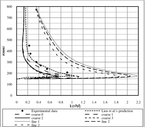
The predicted TKE profiles at x=0.5H for three different turbulence models are compared with wind tunnel data [8] and numerical predictions [7], as illustrated in Fig. 2. TKE profiles of k-ω model lie to the far right whereas those of RSM show reasonable agreement with experimental data. However, the k-ε model (Coarse 0) produces the best agreement. k-ω had an error of 138% as compared to RSM at
45% and k-ε at 21%. Hence, the standard k-ε turbulence model was chosen for subsequent numerical studies.
Fig. 2: TKE curves predicted by various turbulence models and grids at x=0.075m
B. Grid Resolution
[image:2.595.43.248.139.199.2]Further grid refinements are made, as shown in Fig. 3, such that larger mesh densities are concentrated in regions of higher solution gradients, thus allowing better computational resolution.
[image:2.595.307.552.419.507.2]Fig. 3: Meshing for two-dimensional computational model
Fig. 4: TKE curves for various grids at x=0.375m (2.5H) for Case 1
0 100 200 300 400 500 600 700 800
0 0.2 0.4 0.6 0.8 1 1.2 1.4 1.6 1.8 2 2.2
z(
m
m
)
Experimental data Lien et al.'s prediction
coarse 0 coarse 1
coarse 2 coarse 3
fine 1 fine 2
fine 3
0 100 200 300 400 500 600 700 800
0 0.2 0.4 0.6 0.8 1 1.2
z(
m
m
)
Experimental data Lien et al.'s prediction
coarse grid normal grid
fine grid concentrated grid
Velocity inlet
Symmetry
[image:2.595.304.550.543.750.2]The TKE results computed using k-ε model on various refined grids at x=0.375m (2.5H) are compared with experimental data in Fig. 4. The concentrated grid reduced the error to 14% from the basic model’s 21%.
IV. NUMERICAL STUDIES
Six obstacle configurations of different ridge heights and separation distances are investigated using k-ε turbulence model with concentrated mesh, as given in Table 2. It should be noted that in all cases, the separation distance, D is equal
[image:3.595.50.551.403.754.2]to the ridge height, H and hence, Case 1 is the basic configuration replicating the model setup of Lien et al. [7]. The same inlet flow conditions obtained from the wind tunnel measurements [8] are employed in the present study.
Table II: Six obstacle configurations
Case No. (Height, Separation)
Case 1 (Lien et al. [7]) (1H, 1D)
Case 2 (2H, 1D)
Case 3 (3H, 1D)
Case 4 (1H, 2D)
Case 5 (1H, 3D)
Case 6 (2H, 3D)
V. RESULTS
A. Effects of Height Variation
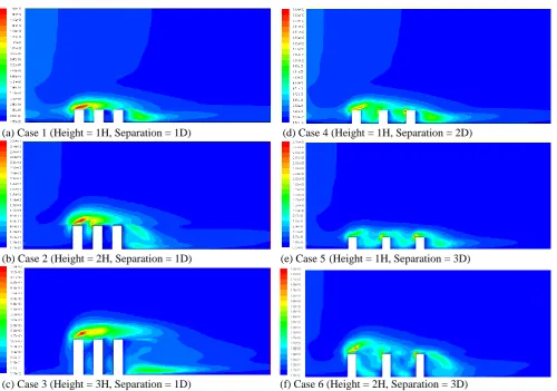
The TKE contour plots for all six cases of varying ridge height and separation are shown in Fig. 5 (a)-(f). Comparison of Figs. 5(a), (b) and (c) shows the effect of increasing ridge heights on TKE over the flow domain and recorded peak TKE values over the leading ridge height, where flow separation occurs, of approximately 1.6, 3.2 and 5.2, respectively.
The flow impingement upwind of the first ridge provokes severe flow curvature over the ridge. The TKE in this region is amplified significantly as a result of the collective effect of streamline curvature as the fluid elements are forced up and over the first ridge. Since the energy is transported by the turbulent boundary layer, the fluid in the inner part of the boundary layer flow has a relatively slower acceleration due to an adverse pressure gradient. Consequently, the fluid is separated from the surface and flow reversal occurs at the top of the ridge, with part of the fluid particle being transported further whereas the remainder contributes to the recirculation eddies between ridges.
In general, there is greater accumulation in the turbulence energy generated with increasing ridge heights. Moving downstream from the top of the first ridge, the downstream variation of the TKE observed is due to mixing turbulent flow layer between ridges. Increasing the ridge height generates greater TKE due to the intensified development of thin intense shear layers along and over the top of the ridge.
(a) Case 1 (Height = 1H, Separation = 1D) (d) Case 4 (Height = 1H, Separation = 2D)
(b) Case 2 (Height = 2H, Separation = 1D) (e) Case 5 (Height = 1H, Separation = 3D)
Figs. 6(a)-(c) presents TKE for three different ridge heights of 1H, 2H and 3H at three downstream locations (a) x=0.5H, (b) x=1.5H and (c) x=2.5H, with the vertical distance, z, non-dimensionalised by respective ridge height.
Since TKE distribution is affected by pressure or advection and turbulent transport from the shear layer, there is a lesser amount of turbulent kinetic energy to be transported further downstream. Comparing peak TKE values between Fig. 6(a)-(c), it can be observed that TKE decreases downstream more significantly from mid-position of the 1st ridge to mid-position between the 1st and 2nd ridge and then decreases more gradually further downstream.
(a) x=0.5H (at mid-position of the 1st ridge)
(b) x=1.5H (at mid-position between 1st & 2nd ridge)
(c) x=2.5H (at mid-position of the 2nd ridge) Figs. 6(a)-(c): TKE for ridges of varying heights
B. Effects of Separation Variation
The TKE contour plots for increasing ridge separation for a fixed height are shown in Figs. 5(c), (d) and (c). Peak TKE recorded at the ridge height where flow separation occurs are approximately 1.6, 1.9 and 3.1, respectively.
Invariably, with increasing separation distances, variation in flow patterns such as flow separation, recirculation and reattachment are evident over a greater downstream extent.
Fig. 7(a)-(c) presents the TKE profiles computed at three locations for 1D, 2D and 3D separation of 1H ridge.
As expected, there is little change in the approach flow characteristics and hence the TKE values at the first ridge [Fig. 7(a)]. The observed large peak in the TKE magnitude seen in Figs. 7(b) and(c) just above the point of separation can be interpreted as an effect arising from an oscillation of the elevated shear layer by the larger-scale upstream turbulence that enhances the concentration of TKE.
However, unsteadiness in the flow pattern is observed in flow region between the first and second ridge [Fig. 7(b)], where recirculation and bubbles of eddies are evident. As a result of greater free space between the ridges as separation increases, the fluid particles are circulated over a larger region leading to a reduced concentration of the TKE, as can been observed in Fig. 7(a)-(c). As the peak TKE soothes downstream, the TKE is distributed along a larger flow domain, decreasing the overall value. However, as the flow proceeds, the TKE that is dispersed seems to recollect to a greater amount as can be seen by the increasing peak value for the 2D and 3D separations. The qualitative features of the flow, showing a successive decrease in the TKE, are the consequences of turbulent dissipation.
(a) at mid-position of the 1st ridge
(b) at mid-position between 1st and 2nd ridges 0
1 2 3 4
0 0.5 1 1.5 2 2.5 3 3.5 4 4.5
z
n
on
d
im
en
sion
al
is
ed
b
y
rid
ge
h
eigh
t
Ridge Height=1H =2H =3H
0 1 2 3 4
0 0.5 1 1.5 2 2.5 3 3.5 4
z
n
on
d
im
en
sion
al
is
ed
b
y
rid
ge
h
eigh
t
Ridge Height=1H =2H =3H
0 1 2 3 4
0 0.5 1 1.5 2 2.5 3 3.5 4
z
n
on
d
im
en
sion
al
is
ed
b
y
rid
ge
h
eigh
t
Ridge Height=1H =2H =3H
0 100 200 300 400 500 600 700 800
0 0.2 0.4 0.6 0.8 1 1.2 1.4 1.6 1.8
z(
m
m
)
k (m2/s2)
Ridge Separation=1D =2D =3D
0 100 200 300 400 500 600 700 800
0 0.2 0.4 0.6 0.8 1 1.2 1.4
z(
m
m
)
(c) at mid-position of the 2nd ridge
Figs. 7(a)-(c): TKE for 1H ridges of varying separation
C. Effects of Height and Spacing Variation
[image:5.595.47.289.48.221.2]Four cases showing the combined effects of variation in height and separation are tabulated in Table 3, with their respective TKE contour plots presented in Fig. 5.
Table III:Variation of height and separations of the ridges.
Case No.
(Height, Separation)
TKE Contour Plots
Case 1 (1H, 1D) Fig. 5 (a)
Case 2 (2H, 1D) Fig. 5 (b)
Case 3 (1H, 3D) Fig. 5(e)
Case 6 (2H, 3D) Fig. 5(f)
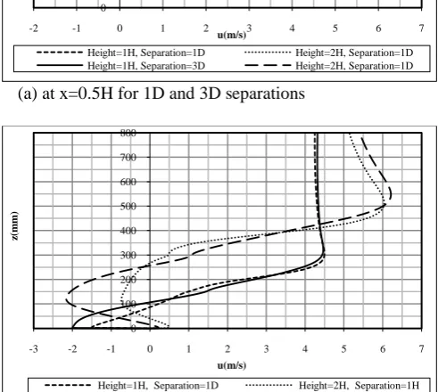
Figs. 8(a)-(c) show the velocity profiles for 1H and 2H ridges at corresponding downstream locations.
Fig. 8(a) illustrates that separation bubbles are captured at mid-point, on top of the first ridge for both 1H and 2H ridges. All profiles show a significant increase in mean velocity across the flow separation region to a maximum value at a level of 5/3H before gradually decreasing to a free stream value. As expected, a larger maximum flow velocity is observed for the 2H due to flow amplification and greater blockage effects when doubling the ridge height. However, the effects of increasing separation for both ridge heights at the first-ridge location are minimal.
Fig. 8(b) shows the velocity profiles in-between the 1st and 2nd ridges where street canyon effects are strongly evident. Stronger recirculating flows are seen for the higher ridge. Larger ridge separation has a mitigating effect of reducing the vortex strength in-between the ridges. A vital feature captured by the model in Fig. 8(b) is the formation of a shear layer downstream of the rear face of the first ridge, as revealed by the inflection point and flow reversal.
In Fig. 8(c), velocity profiles at mid-point on the top of the second ridge show no reverse flow. Ridge separation affects mean flow more significantly from this point onwards as greater separation allows flow relaxation in between the first and the second ridge [c.f. TKE contour plots of Fig. 5(b) and (f)].
(a) at x=0.5H for 1D and 3D separations
(b) at x=1.5H for 1D separations and x=2.5H for 3D separations
(c) at x=2.5H for 1D separations and x=4.5H for 3D separations
Fig. 8(a)-(c): Velocity profiles for ridges of varying heights and separation
Fig. 9(a) and (b) show the comparisons of TKE profiles for two ridge heights (1H, 2H), each for two separations (1D, 3D), at mid-point position of the 2nd ridge and mid-position in-between the 2nd and the 3rd ridge element, respectively.
In Fig. 9(a), TKE peaks are observed for all cases. Increasing ridge height from 1H to 2H for 1D separation doubled the maximum TKE values. However, the increase in TKE is only marginal for the two 3D separations where both ridge heights registered lower TKE peak values. There is a 0
100 200 300 400 500 600 700 800
0 0.2 0.4 0.6 0.8 1 1.2 1.4
z(
m
m
)
Ridge Separation=1D =2D =3D
0 100 200 300 400 500 600 700 800
-2 -1 0 1 2 3 4 5 6 7
z(
m
m
)
u(m/s)
Height=1H, Separation=1D Height=2H, Separation=1D Height=1H, Separation=3D Height=2H, Separation=1D
0 100 200 300 400 500 600 700 800
-3 -2 -1 0 1 2 3 4 5 6 7
z(
m
m
)
u(m/s)
Height=1H, Separation=1D Height=2H, Separation=1H Height=1H, Separation=3D Height=2H, Separation=3D
0 100 200 300 400 500 600 700 800
-1 0 1 2 3 4 5 6 7
z(
m
m
)
u(m/s)
[image:5.595.305.551.50.208.2] [image:5.595.305.551.168.388.2]halfing in TKE for the 2H ridge when the separation is increased from 1D to 3D, but not for the shorter ridge height of 1H.
Fig. 9(b) captures similar trend in TKE peak values between 1D and 3D separation for both ridge heights but with strong influence of recirculating flows in-between the two ridges, particularly for ridge height of 2H.
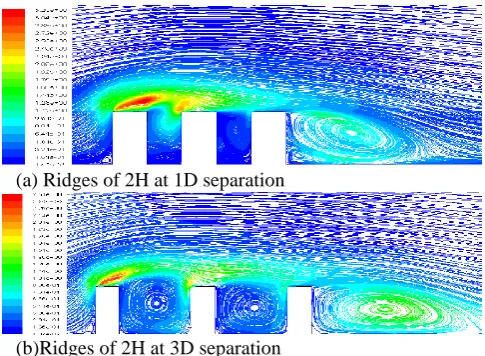
Results of Figs. 9(a) and (b) for 2H ridge height are elucidated further by observing the flow pathlines (colored by TKE values) of Figs. 10(a) and (b).
For 2H ridge, the wider 3D separation allows significant flow development (street canyon effects) in-between ridges, whereas for the narrower distance of 1D, stronger interaction with flow separation and reattachment from the top leading edge of the first ridge is seen in-between the first two ridges, though street canyon effects are also evident.
It is interesting to note that for 1H ridge height, increasing separation from 1D to 3D increases TKE peak values, as opposed to a decrease in the case of the 2H ridge height.
In summary, varying ridge height and separation of an array of three parallel ridges produces different and rather complex interactions of upwind flow separation and recirculation around the ridges as observed by the TKE profiles and peak TKE values in Figs. 8 and 9.
(a) at x=2.5H for 1D separations and x=4.5H for 3D separations
(b) at x=3.5H for 1D separations and x=6.5H for 3D separations
Fig. 9(a)-(b): TKE profiles for ridges of varying height and separation
(a) Ridges of 2H at 1D separation
(b)Ridges of 2H at 3D separation
Fig. 10(a)-(b): Maps of pathlines (colored by TKE values)
VI. CONCLUSION
Numerical studies of a two-dimensional model of three-parallel ridges in FLUENT based on the inbuilt RANS turbulence models show that the standard k-ε model predicts the flow most accurately in relation to the TKE distribution. Using a two-dimensional domain can reduce the computational demand without compromising the accuracy of predictions when suitable mesh configurations and turbulence model are applied.
Significant variation in TKE is observed when the ridge height and/or separation are varied as depicted by the mean velocity profiles, TKE profiles, and contour maps of TKE. As the flow progresses downstream the overall value of TKE decreases due to energy dissipation. An amplification of the velocity and TKE are observed as the ridge height increases, whereas larger separations result in lower velocities and significant variation in downwind TKE values that are dependent on the ridge height.
REFERENCES
[1] D.A. Paterson, and C.J. Apelt, “Computation of wind flows over three-dimensional buildings,” J. Wind Eng. And Ind. Aerodynamics, vol. 24, 1986, pp. 193-213.
[2] Y.Q. Zhang, A.H. Huber, S.P.S. Arya, and W.H. Synder, “Numerical Simulation to determine the effects of incident wind shear and turbulence on the flow around a building,’’ J. Wind Eng. And Ind. Aerodynamics, vol. 46-47, 1993, pp. 129-134.
[3] Y. Zhou, and T. Stathopoulos, “A new technique for the numerical simulation of wind flow around buildings,” J. Wind Eng. And Ind. Aerodynamics, vol. 72, 1997, pp. 137-147.
[4] I.R. Cowan, I.P. Castro and A.G. Robins, “Numerical considerations for simulations of flow and dispersion around buildings,” J. Wind Eng. Ind. Aerodynamics., vol. 67–68, 1997, pp. 535–545.
[5] Y. Alexander, H. Liu, and N. Nikitin, “Turbulent flow around a wall mounted cube: A direct numerical simulation,” Int. J. Heat and Mass Transfer, vol. 27, 2006, pp. 994-1009.
[6] G.S. Ratnam, and S. Vengadesan, “Performance of two equation turbulence models for prediction of heat transfer over a wall mounted cube,” Int. J. Heat and Mass Transfer, vol. 51, 2008, pp. 2834-2846. [7] F.S. Lien, E. Yee, and Y. Cheng, “ Simulation of mean flow and
turbulence over a 2D building array using high resolution CFD and a distributed drag flow approach,” J. Wind Eng. And Ind. Aerodynamics, vol. 92, 2004, pp. 117-158.
[8] M.J. Brown, R.E. Lawson, D.S. Decroix, and R.E. Lee, “Comparison of centerline velocity measurements obtained around 2D and 3D building arrays in a wind tunnel”, Report LA-UR-01-4138, Los Alamos National Laboratory, Los Alamos, 2000.
0 100 200 300 400 500 600 700 800
0 0.2 0.4 0.6 0.8 1 1.2 1.4 1.6 1.8 2 2.2 2.4
z
(m
m
)
k (m2/s2)
Height=1H, Separation=1D Height=2H, Separation=1D Height=1H, Separation=3D Height=2H, Separation=3D
0 100 200 300 400 500 600 700 800
0 0.2 0.4 0.6 0.8 1 1.2 1.4 1.6
z
(m
m
)
k (m2/s2)
[image:6.595.307.550.48.226.2]