Single Seven State Discrete Time Extended Kalman Filter for Micro Air Vehicle

(1)

Single Seven State Discrete Time Extended

Kalman Filter for Micro Air Vehicle

Dr. Afzaal M. Malik1_{and Sadia Riaz}2

Abstract—The term Micro Air Vehicles (MAVs) is used for a new type of remotely controlled, semi-autonomous or autonomous aircraft that is significantly smaller than conventional aircrafts. To apply Micro Electro Mechanical Systems (MEMS) inertial sensors for the Guidance, Navigation and Control (GNC) of Micro Air Vehicle (MAV) is an extremely challenging area. The major components of the control system of micro air vehicles are the onboard sensors. This paper presents an approach for the implementation of on board sensors for Micro Air Vehicles and the application of a Seven State Discrete Time Extended Kalman Filter. On-board sensors are linked to the Ground Control Station (GCS). This paper presents an approach of applying an Inertial Navigation System (INS) using MEMS inertial sensors and Global Positioning System (GPS) receiver with a Single Seven State Discrete Time Extended Kalman Filter. Inertial navigation system (INS) includes MEMS gyro, accelerometer, magnetometer and barometer. MEMS inertial sensors are of utmost importance in the GNC system. The system considered is non-linear and it is first linearized for application of the Kalman Filter. A Single Seven State Discrete Time Extended Kalman Filter is used for state estimation. Process covariance matrix and measurement covariance matrix are derived.

Index Terms— Micro Electro Mechanical System (MEMS),

Micro Air Vehicle (MAV), Measurement Covariance Matrix, Process Covariance Matrix

Nomenclature

Inertial North Position of MAV Inertial East Position of MAV Wind from North

Wind from East Total Airspeed

Angular Rate about x-axis Angular Rate about y-axis Angular Rate about z-axis Roll Angle

Pitch Angle Yaw Angle

Manuscript received January 28,2010. this work was supported by College of Electrical and Mechanical Engineering, National University of Sciences and Technology (NUST). Financial Support was provided by Higher Education Commission, Pakistan.

Dr. Afzaal M. Malik is a Professor in the Department of mechanical Engineering (DME), College of Electrical and Mechanical Engineering (CEME), National University of Sciences and Technology (NUST), Rawalpindi, Pakistan.(drafzaalmalik@ceme.nust.edu.pk)

Sadia Riaz2_{(correspondence author) is a graduate student in the} Department of Mechanical Engineering (DME), College of Electrical and Mechanical Engineering (CEME), National University of Sciences and Technology (NUST), Rawalpindi, Pakistan. (sadia_shhzd@yahoo.com)

• As superscript shows the rate of change Northern Magnetic Field Component Eastern Magnetic Field Component Vertical Magnetic Field Component Process Covariance Noise Matrix Process Covariance Noise Matrix

I. INTRODUCTION

By Defense Advanced Research Projects Agency (DARPA) standards [1], a Micro Air Vehicle (MAV) is limited to a maximum dimension of 15 cm, gross weight of 100 g, with up to 20 g payload and the Reynolds number must be below 106_[2]_{. The size limitation for MAV for}

International MAV competitions is 100 cm for outdoor missions and 70/80 cm for indoor missions with maximum weight of 1 kg [3]. In MAV configuration, the dimension of 15 cm is very critical because it is considered border line between bird flight and insect flight [4]. The flight-control algorithms used for MAVs have been primarily based on the Radio Controller (R/C) or Tele-Operation [5]. Guidance, Navigation and Control (GNC) has been an important area in MAV research. On-board sensors (MEMS gyro, MEMS accelerometer, Magnetometer and GPS) have crucial importance in GNC. These sensors are used for state estimation of MAV. In this paper an approach of Single Seven State Discrete Time Extended Kalman Filter is used for the state estimation of MAV.

II. GUIDANCE AND FLIGHT CONTROL LOOP

The guidance loop [6,7] is an outer control loop in autonomous flight mode. It computes guidance demands to force the vehicle to follow the desired way-point to reach the destination. The guidance loop provides the guidance demands from the current vehicle states and the next way-point information. The guidance demands are the desired vehicle speed with respect to the air, the desired height and the bank angle.

R Q moz moy m_ox

ψ θ φ r q p V W W P P

[image:1.595.312.549.679.755.2]

air E N E N

(2)

The flight control loop [8] caters for the vehicle’s attitude and attitude rates as well as the vehicle speed with respect to the air. It performs speed control, height control, bank angle control, heading control and elevation control by using the guidance demands and the measured vehicle states. It generates actuator signals for the engine throttle, rudder, elevator and aileron. The proposed flight control system is shown in figure 02.

III. SINGLE 7STATE DISCRETE TIME EXTENDED KALMAN

FILTER STATE ESTIMATION SCHEME

The Discrete Time [9] Extended Kalman Filter (EKF) considers discrete-time dynamics and discrete-time measurements. This situation is often considered in practice. Even if the underlying system dynamics are continuous time, the EKF usually needs to be implemented in a digital computer. This means there might not be enough computational power to integrate the system dynamics as required in a continuous-time [9] EKF or a hybrid [9] EKF. So the dynamics are often discretized [9] and then discrete-time EKF can be used.

The state equations which relate body frame rotations to changes in roll, pitch and heading are nonlinear. Letting the states be roll angle (ϕ) and pitch angle (θ), and letting angular rates (p, q and r) and Airspeed

V

_air be inputs.

The update of the states is related to the inputs as shown below [10]

:

The linearization of Extended Kalman Filter through Jacobian method [11]

⎥ ⎥ ⎥ ⎥ ⎥ ⎥ ⎥ ⎥ ⎥ ⎥

⎦ ⎤

⎢ ⎢ ⎢ ⎢ ⎢ ⎢ ⎢ ⎢ ⎢ ⎢

⎣ ⎡

+ + + + + +

=

⎥ ⎥ ⎥ ⎥ ⎥ ⎥ ⎥ ⎥ ⎥

⎦ ⎤

⎢ ⎢ ⎢ ⎢ ⎢ ⎢ ⎢ ⎢ ⎢

⎣ ⎡

0 0 sin cos cos

cos cos

sincos sin tan cos tan

sin

E air

N air

E N E N

W V

r q

p

W W P P

ψ

ψ θ

φ θ

φφ φ

θ φ θ

φ

ψ θ φ

⎥ ⎥ ⎥ ⎥ ⎥ ⎥ ⎥ ⎥ ⎥ ⎥ ⎥

⎦ ⎤

⎢ ⎢ ⎢ ⎢ ⎢ ⎢ ⎢ ⎢ ⎢ ⎢

⎣

− − +

− + − = ∂ ∂

0 0 0 0 0 0

0

0 0 0 0 0 0

0

1 0 0 0 0 0

0

0 1 0 0 0 0

0

0 0 0 0 0 tan sec ) cos sin ( cos sin cos cos

0 0 0 0 0 0

cos

sin cos cos

) ,

( _θφ _θφ φ φ θ θ

φ φ

r q r

q r q

x u x f

⎢

⎡ ₋ sin ₊ cos ₀ ₀ ₀ ₀ ₀

tan sin tan

cos ₂ ₂

θ φ θ φ θ

φ θ

φ r q r

q

Measurement

The linearization of Extended Kalman Filter through Jacobian method [11]

E N E N

W W P P ψ θ φ

[image:2.595.54.542.50.257.2]

Fig. 3 Single Seven State Extended Kaman Filterscheme

Fig. 2 Proposed Control System

( )

( ) ( )

⎥ ⎥ ⎥ ⎥ ⎥ ⎥ ⎥ ⎥ ⎥ ⎥ ⎥ ⎥ ⎥ ⎥

⎦ ⎤

⎢ ⎢ ⎢ ⎢ ⎢ ⎢ ⎢ ⎢ ⎢ ⎢ ⎢ ⎢ ⎢ ⎢

⎣ ⎡

+ −

+ +

+ −

− +

− −

+

=

E N

oz oy

ox

oz oy

ox

oz oy ox

air air

air

P P

m m

m

m m

m

m m m

g q V

g r r V

g q V

u x h

θ φ ψ φ ψ θ φ ψ φ ψ θ φ

θ ψ θ ψ θ

φ θ θ

φ θ θ θ

θ θ

cos cos cos sin sin sin cos sin sin cos sin cos

cos sin cos cos sin sin sin sin cos cos sin sin

sin sin cos cos cos

sin cos cos

cos cos sin cos

sin sin

,

(3)

The Process Covariance Matrix [12,13] is given as follows:

The Measurement Covariance Matrix [12,13] is given as follows:

( )

(

)

(

)

(

)

(

)

(

₍

)

₎

(

)

(

)

(

)

(

₍

)

₎

⎥ ⎥ ⎥ ⎥ ⎥ ⎥ ⎥ ⎥ ⎥ ⎥ ⎥ ⎥ ⎥ ⎥ ⎥ ⎥ ⎥ ⎥ ⎥ ⎥ ⎥ ⎥ ⎥ ⎦ ⎤ ⎢ ⎢ ⎢ ⎢ ⎢ ⎢ ⎢ ⎢ ⎢ ⎢ ⎢ ⎢ ⎢ ⎢ ⎢ ⎢ ⎢ ⎢ ⎢ ⎢ ⎢ ⎢ ⎢ ⎣ ⎡ + + + − − + − − + + − − + − − + + + − + + + − − − − + + + − − + = ∂ ∂ = 1 0 0 0 0 0 1 0 0 0 0 0 sin sin cos cos cos cos sin sin sin cos sin cos sin cos cos cos cos cos cos sin cos cos sin sin cos sin cos cos sin sin 0 0 sin cos cos sin sin cos cos sin sin sin sin sin sin cos sin sin cos sin cos cos cos sin sin sin cos ) sin sin cos sin (cos 0 0 cos cos sin cos cos sin sin cos sin 0 0 0 0 cos sin sin sin cos 0 0 0 sin sin ) cos sin ( cos cos 0 0 0 cos cos 0 , 0 oy ox oz oy ox oz oy ox oy ox ozz oy ox oz oy ox oy ox oz y ox air air air m m m m m m m m m m m m m m m m m m m m m g q V g p r V g q V x u x h C ψ φ ψ θ φ ψ φ ψ θ φ θ φ ψ θ φ ψ θ φ θ φ ψ φ ψ θ φ ψ φ ψ θ φ ψ φ ψ θ φ ψ φ ψ θ φ θ φ ψ θ φ ψ θ φ θ φ ψ φ ψ θ φ ψ φ ψ θ φ ψ θ ψ θ θ φ θ ψ θ φ θ θ φ θ φ θ θ θ φ θ θ θ

( )

T

(4)

IV. RESULT AND ANALYSIS

0 2 4 6 8 10 12 14 16 18

-1 -0.8 -0.6 -0.4 -0.2 0 0.2 0.4

Velocity in Z-Direction Versus Accelerometer Output

w (m/s)

ac

c

le

ra

ti

o

n (

m

/s

2)

[image:4.595.307.541.53.212.2]

ax actual ax estimated ay actual ay estimated az actual az estimated

Fig. 6 Velocity in Z-Direction Versus Accelerometer Output

[image:4.595.50.283.172.339.2]

The output of the on-board sensors is mathematically modeled and filtered with the help of Single Seven State Discrete Time Extended Kalman Filtering. The graphs are based on the linearized equations of motion that also take into account the rotation of the body frame with respect to the inertial frame. The actual and estimated results are compared as following:

Fig. 4 Velocity in X-Direction Versus Accelerometer Output

0 5 10 15 20 25 30

-1.2 -1 -0.8 -0.6 -0.4 -0.2 0 0.2 0.4

Velocity in X-Direction Versus Accelerometer Output

u (m/s)

ac

ce

le

rat

ion (

m

/s

2 )

ax actual ax estimation ay actual ay estimation az actual az estimation

Since velocity does not have any impact on the states, a variation in velocity in the x direction would not indirectly cause major inaccuracies in the measurements. There is, however, slight inaccuracy in the x direction acceleration owing to the fact that the state estimate appears uncoupled in the formula and therefore has a greater impact on the measurement of acceleration in the x direction than in the other directions.

Variation in velocity in the y direction has no effect on acceleration in the y direction, whereas it does on accelerations in the other two axes. Single State Kalman Filter show almost the same accuracy in the case of variable velocity in y direction as for variable velocity in x direction.

As cited earlier, variation in velocity in the z direction has no effect on acceleration in the z direction whereas it does on acceleration in the other two axes. Single State Kalman Filter again showed the same accuracy as it did for variable velocity in x and y in the previous graphs.

0.6

In above figure the Kalman filter estimates of the measurement of acceleration show increased inaccuracy owing to the dependence of the states (Euler angles) being used in measurement, on the angular rates. The curves are oscillatory in nature owing to the presence of the indirect effect of process noise that is passed on in the state estimates.

0 2 4 6 8 10 12 14 16 18 20

-0.8 -0.6 -0.4 -0.2 0 0.2 0.4

0.6 Velocity in Y-Direction Versus Accelerometer Output

v (m/s)

ac

cl

er

at

io

n (

m

/s

2)

[image:4.595.307.547.313.464.2]

Fig. 5 Velocity in Y-Direction Versus Accelerometer Output

-0.2 -0.15 -0.1 -0.05 0 0.05 0.1 0.15 0.2

-1 -0.5 0 0.5 1 1.5 2

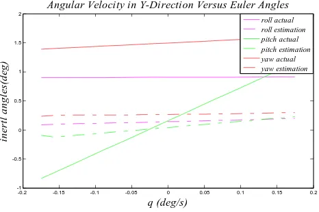
Angular Velocity in Y-Direction Versus Euler Angles

q (deg/s)

in

er

tl

a

n

g

le

s(

d

eg

)

roll actual roll estimation pitch actual pitch estimation yaw actual yaw estimation

Fig. 8 Angular Velocity in Y-Direction Versus Accelerometer Output

-0.4 -0.3 -0.2 -0.1 0 0.1 0.2 0.3

-0.8 -0.6 -0.4 -0.2 0 0.2 0.4

Angular Rate in X-Direction Versus Accelerometer Output

p (deg/s)

a

ccel

er

a

ti

o

n

(

m

/s

ax actual ax estimation ay actual ay estimation az actual

2 )

az estimation

[image:4.595.49.276.473.633.2] [image:4.595.309.542.590.745.2]

(5)

[image:5.595.320.542.53.208.2]

Figure. 8 shows variation in acceleration owing to changes in the angular rate about the y axis. Angular rate about the y axis only affects acceleration in the x and z axes. As for the Kalman Filter estimates, they are still quite inaccurate owing to the dependence of the state estimate on the value of angular rates.

-0.2 -0.15 -0.1 -0.05 0 0.05 0.1 0.15 0.2

-1 -0.5 0 0.5 1 1.5 2

Angular Velocity in Y-Direction Versus Euler Angles

q (deg/s)

E

ule

r Angl

es(

de

g)

Fig. 11 Angular Velocity in Y-Direction Versus Euler Angles

-0.4 -0.3 -0.2 -0.1 0 0.1 0.2 0.3 0.4

-2 -1.5 -1 -0.5 0 0.5

Angular Velocity in Z-Direction Versus Accelerometer Output

r (deg/s)

ac

ce

le

rat

io

n (

m

/s

2 )

[image:5.595.44.267.143.300.2]

Fig. 9 Angular Velocity in Z-Direction Versus Accelerometer Output

The above graph shows variation in acceleration owing to changes in the angular rate about the z axis. Angular rate about the z axis affects only the acceleration in the x and y axes. As for the single Kalman filter estimates, they are still quite inaccurate owing to inaccuracies in the state estimates.

The above graph shows variation in inertial angles with respect to change in angular rate about x axis. Since the transformation about the x axis is the last in the sequence of transformations, the Euler angle in the x axis almost matches the body angular rate in the same axis. The other angular rates remain constant with changes in the body angular rate around x axis, since this is the last step of the transformation and therefore the orthogonal axes have become independent of the influence of any further transformations. The single step Kalman filter estimate is not very inaccurate, except for the oscillations due to the presence of noise.

The second graph shows variation in Euler angles with respect to changes in angular rate about the y axis. All Euler angles are dependent on the body angular rate about y axis to a certain extent, owing to the fact the transformation about y axis is the second in the sequence. But it is Euler angle about y axis that shows the largest variation with change in q. This variation has a simple linear character when the Euler angle in the x axis is small. The single step Kalman filter, as before, is quite accurate.

2.5

The above graph shows variation in Euler angles with respect to change in angular rate about z axis. Since the transformation about z axis is the first in the sequence of single transformations, all Euler rates are affected by change in the dynamics of the z axis. Euler angular rate about z axis is the most affected because of the relationship between the same axes. The relationship is dependent on primarily the pitch angle. The single step Kalman Filter is quite accurate.

-0.4 -0.3 -0.2 -0.1 0 0.1 0.2 0.3

-1.5 -1 -0.5 0 0.5 1 1.5 2

Angular Velocity in X-Direction Versus Euler Angles

p (deg/s)

Eul

e

r Angl

es

(d

eg

)

[image:5.595.308.547.403.575.2]

Fig. 10 Angular Velocity in X-Direction Versus Euler Angles

-0.4 -0.3 -0.2 -0.1 0 0.1 0.2 0.3 0.4

-2 -1.5 -1 -0.5 0 0.5 1 1.5 2

Angular Velocity in Z-Direction Versus Euler Angles

r (deg/s)

Eu

le

r An

g

le

s(

d

eg

)

[image:5.595.39.280.432.588.2]

(6)

V. CONCLUSIONS

The MAV could provide significant new capabilities to a wide range of users. Several MAVs and a base station could be transported and operated by a single individual, providing real-time data directly to the local user. The MAV promises to be particularly useful for covert operations. Application of Single Seven State Discrete Time Extended Kalman Filter is helpful in state estimation.

VI. ACKNOWLEDGEMENTS

The authors are indebted to the College of Electrical and Mechanical Engineering (CEME), National University of Sciences and Technology (NUST), Higher Education Commission (HEC) and Pakistan Science Foundation (PSF) for having made this research possible.

REFERENCES

[1] James M. McMichael (Program Manager Defense Advanced Research Projects Agency) and Col. Michael S. Francis, USAF (Ret.) (Defense Airborne Reconnaissance Office), “Micro air vehicles - Toward a new dimension in flight” dated 8/7/97 [2] B-J Tsahi, Y-C Fu, “Design and aerodynamic

analysis of flapping wing micro air vehicle ”, Aerospace Science and Technology 2009, AESCTE-2474

[3] International Micro Air Vehicle Competition, to be held on 6-8 Jul 2010 at Braunschwieg, Germany. http://www.imav.com accessed on 25 January 2010 [4] Ho, Hany Nassel, Nick Pornisinsirirak, Yu-Chong Tai and Chih-Ming Ho, “Unsteady aerodynamics and flow control for flapping wing flyers” Progress in Aerospace Sciences 2003, Vol. 39, pp 635-681.

[5] “Ground control station development for

autonomous UAV ”by Ye Hong, Jiancheng Fang, and Ye Tao. Key Laboratory of Fundamental Science for National Defense, Novel Inertial Instrument & Navigation System Technology, Beijing, 100191, China

[6] “Integration of GPS/INS/Vision sensors to navigate unmanned aerial vehicles” by Jinling Wanga, Matthew Garrattb_{, Andrew Lambert}c_{, Jack Jianguo}

Wang a_{, Songlai Han}a_{, David Sinclair}d_.a _{School of}

Surveying & Spatial Information Systems, University of New South Wales, NSW 2052, Australia (Jinling.Wang@unsw.edu.au). b_School

of Aerospace, Civil and Mechanical Engineering. c

School of Information Technology and Electrical Engineering, Australia Defence Force Academy,

Canberra, Australia. d _{QASCO Surveys Pty.}

Limited, 41 Boundary St. South Brisbane, Qld, 4101, Australia.

[7] “Development of a flight avionics system for an autonomous micro air vehicle” By Jason Plew, a thesis presented to the graduate school of the University of Florida in partial fulfillment of the requirements for the degree of master of science, University of Florida, 2004.

[8] “Integration of MEMS inertial sensor-based GNC of a UAV” by Z. J. Huang and J. C. Fang (huangzhongjun@buaa.edu.cn,fangjiancheng@b uaa.edu.cn) from School of Instrumentation & Optoelectronics Engineering Beihang University, Beijing 100083, China. International Journal of Information Technology. Vol. 11 No. 10 2005 (pg 123-132)

[9] “Optimal state estimation Kalman, and nonlinear approaches” by Dan Simon, Cleveland State University. A John Wiley &Sons, INC., Publication.

∞

H

[10] “State estimation for micro air vehicles” by Randal W. Beard, Department of Electrical and Computer Engineering, Brigham Young University, Provo, Utah. Studies in Computational Intelligence (SCI) 70, 173–199 (2007). Springer-Verlag Berlin Heidelberg 2007

[11] Elbert Hendricks, Ole Jannerup, Paul Haase Sorensen, “Linear Systems Control” Deterministic and Stochastic Method, ISBN: 978-3-540-78485-2, Library of Congress Control Number: 208927517, 2008 Springer-Verlag Berlin Heidelberg.

[12] “Kalman filtering theory and practice” by Grewal, M. and A. Andrews. Englewood Cliffs, NJ: Prentice-Hall, 1993.

[13] “Applied optimal estimation” Gelb, A. Cambridge, MA: MIT Press, 1974.