Speed-Accuracy Tradeoffs in Tagging
with Variable-Order CRFs and Structured Sparsity
Tim Vieira∗and Ryan Cotterell∗and Jason Eisner
Department of Computer Science Johns Hopkins University
{timv,ryan.cotterell,jason}@cs.jhu.edu
Abstract
We propose a method for learning the structure of variable-order CRFs, a more flexible variant of higher-order linear-chain CRFs. Variable-order CRFs achieve faster inference by in-cluding features for only some of the tagn -grams. Our learning method discovers the useful higher-order features at the same time as it trains their weights, by maximizing an objective that combines log-likelihood with a structured-sparsity regularizer. An active-set outer loop allows the feature set to grow as far as needed. On part-of-speech tagging in5 randomly chosen languages from the Universal Dependencies dataset, our method of shrink-ing the model achieved a2–6x speedup over a baseline, with no significant drop in accuracy.
1 Introduction
Conditional Random Fields (CRFs) (Lafferty et al., 2001) are a convenient formalism for sequence label-ing tasks common in NLP. A CRF defines a feature-rich conditional distribution over tag sequences (out-put) given an observed word sequence (in(out-put).
The key advantage of the CRF framework is the flexibility to consider arbitrary features of the input, as well as enough features over the output structure to encourage it to be well-formed and consistent. How-ever, inference in CRFs is fast only if the features over the output structure are limited. For example, an order-kCRF (or “k-CRF” for short, withk >1
being “higher-order”) allows expressive features over a window ofk+1adjacent tags (as well as the input),
and then inference takes timeO(n·|Y|k+1), where Y is the set of tags andnis the length of the input.
How large does kneed to be? Typicallyk = 2
works well, with big gains from0→1and modest
∗Equal contribution
0 1000 2000 3000 4000 5000 Number of Tag String Features
91 92 93 94 95 96 97 98
Accuracy 0-CRF
[image:1.612.321.536.198.337.2]1-CRF Bulgarian2-CRF Norwegian Hindi Slovenian Basque
Figure 1: Speed-accuracy tradeoff curves on test data for the5languages. Large dark circles represent thek -CRFs of ascending orders along x-axis (marked on for Slovenian). Smaller triangles each represent a VoCRF discovered by sweeping the speed parametersγ. We find faster models at similar accuracy to the bestk-CRFs (§5).
gains from1→2(Fig. 1). Smallkmay be sufficient
when there is enough training data to allow the model to attend to many fine-grained features of the input (Toutanova et al., 2003; Liang et al., 2008). For ex-ample, when predicting POS tags in morphologically-rich languages, certain words are easily tagged based on their spelling without considering the context (k= 0). In fact, such languages tend to have a more
free word order, making tag context less useful. We investigate a hybrid approach that gives the accuracy of higher-order models while reducing run-time. We build on variable-order CRFs (Ye et al., 2009) (VoCRF), which support features on tag sub-sequences of mixed orders. Since only modest gains are obtained from moving to higher-order models, we posit that only a small fraction of the higher-order features are necessary. We introduce a hyperparam-eterγ thatdiscouragesthe model from using many higher-order features (= faster inference) and a hy-perparameterλthatencouragesgeneralization. Thus,
sweeping a range of values forγandλgives rise to a
number of operating points along the speed-accuracy curve (triangle points in Fig. 1).
We present three contributions: (1)A simplified
exposition of VoCRFs, including an algorithm for computing gradients that is asymptotically more ef-ficient than prior art (Cuong et al., 2014). (2)We
develop a structure learning algorithm for discover-ingthe essential set of higher-order dependencies so that inference is fastandaccurate. (3)We investigate
the effectiveness of our approach on POS tagging in five diverse languages. We find that the amount of required context for accurate prediction is highly language-dependent. In all languages, however, our approach meets the accuracy of fixed-order models at a fraction of the runtime.
2 Variable-Order CRFs
An order-kCRF (k-CRF, for short) is a conditional
probability distribution of the form
pθ(y|x) =Zθ1(x)expPn+1t=1 θ>f(x, t, yt−k. . . yt)
wherenis the length of the inputx,θ∈Rd is the
model parameter, andf is an arbitrary user-defined
function that computes a vector inRdof features of
the tag substrings=yt−k. . . ytwhen it appears at
positiont of inputx. We define yi to be a
distin-guished boundary tag#wheni /∈[1, n].
A variable-order CRF or VoCRF is a refinement of thek-CRF, in whichf may not always depend on all k+ 1of the tags that it has access to. The features
of a particular tag substring s may sometimes be
determined by a shorter suffix ofs.
To be precise, a VoCRF specifies a finite set
W ⊂ Y∗ that is sufficient for feature computation
(whereY∗denotes the set of all tag sequences).1The
VoCRF’s featurization functionf(x, t,s)is then
de-fined asf0(x, t,w(s))wheref0 can be any function
andw(s)∈Y∗is the longest suffix ofsthat appears
inW (or εif none exists). The full power of ak
-CRF can be obtained by specifyingW =Yk+1, but
smallerW will in general allow speedups.
To support our algorithms, we define W to be the closure ofW under prefixes and last-character
substitution. Formally,Wis the smallest nonempty superset ofWsuch that ifhy ∈ Wfor someh∈Y∗ 1The constructions given in this section assume that
Wdoes not containεnor any sequence having##as a proper prefix.
Algorithm 1FORWARD: ComputelogZθ(x). α(·,·) = 0;α(0,#) = 1 .initialization
fort= 1ton+ 1:
ift=n+ 1thenYt={#}elseyt=Y\{#}
forh∈ H, yt∈Yt: h0 =NEXT(h, yt)
z= exp θ>f0(x, t,w(hyt)) α(t,h0)+=α(t−1,h)·z
Z =Ph∈Hα(n+ 1,h) .sum over final states
returnlogZ
Algorithm 2GRADIENT: Compute∇θlogZθ(x). β(·,·) = 0;∆=0
β(n+ 1,h) = 1for allh∈ H .initialization
fort=n+ 1downto1:
forh∈ H, yt∈Yt: h0 =NEXT(h, yt)
z= exp θ>f0(x, t,w(hyt))
∆+=f0(x, t,w(hyt))·α(t−1,h)·z·β(t,h0) β(t−1,h)+=z·β(t,h0)
return∆/Z
andy ∈Y, thenh ∈ W and alsohy0 ∈ W for all
y0 ∈Y. This implies that we can factorWasH ×Y,
whereH ⊂Y∗is called the set ofhistories.
We now define NEXT(h, y)to return the longest
suffix ofhythat is inH(which may behyitself, or evenε). We may regard NEXTas the transition func-tion of a deterministic finite-state automaton (DFA) with state setHand alphabetY. If this DFA is used to read any tag sequencey∈Y∗, then the arc that reads ytcomes from a statehsuch thathytis the longest
suffix of s = yt−k. . . yt that appears in W—and
thusw(hyt) = w(s) ∈ W and provides sufficient
information to computef(x, t,s).2
For a givenxof lengthnand given parametersθ,
the log-normalizerlogZθ(x)—which will be needed
to compute the log-probability in eq. (1) below—can be found in time O(|W|n) by dynamic
program-ming. Concise pseudocode is in Alg. 1. In effect, this
runs the forward algorithm on the lattice of taggings given by length-npaths through the DFA.
For finding the parametersθthat minimize eq. (1)
below, we want the gradient ∇θlogZθ(x). By
applying algorithmic differentiation to Alg. 1, we obtain Alg. 2, which uses back-propagation to compute the gradient (asymptotically) as fast as Alg. 1 and|H|times faster than Cuong et al. (2014)’s
algorithm—a significant speedup since|H|is often quite large (up to300in our experiments). Algs. 1–2
together effectively run the forward-backward algorithm on the lattice of taggings.3
It is straightforward to modify Alg. 1 to obtain a Viterbi decoder that finds the most-likely tag se-quence underpθ(· |x). It is also straightforward to
modify Alg. 2 to compute the marginal probabilities of tag substrings occurring at particular positions.
3 Structured Sparsity and Active Sets We begin with ak-CRF model whose feature vector f(x, t, yt−k. . . yt)is partitioned into non-stationary
local features f(1)(x, t, yt) and stationary
higher-order features f(2)(yt−k. . . yt). Specifically, f(2)
includes an indicator feature for each tag stringw∈ Y∗ with1 ≤ |w| ≤ k+ 1, wherefw(2)(yt−k. . . yt)
is 1 ifwis a suffix ofyt−k. . . ytand is 0 otherwise.4
To obtain the advantages of a VoCRF, we merely have to choose a sparse weight vector θ. The set
W can then be defined to be the set of strings in
Y∗whose features have nonzero weight. Prior work
(Cuong et al., 2014) has left the construction ofW to domain experts or “one size fits all” strategies (e.g.,
k-CRF). Our goal is to chooseθ—and thusW—so that inference is accurateandfast.
Our approach is to modify the usual L2
-regularized log-likelihood training criterion with a carefully defined runtime penalty scaled by a param-eterγto balance competing objectives: likelihood on
the data{(x(i),y(i))}m
i=1vs. efficiency (smallW).
−
m X
i=1
logpθ(y(i)|x(i))
| {z }
loss
+ λ||θ||22
| {z } generalization
+γR(θ)
| {z } runtime
(1)
Recall that the runtime of inference on a given sentence is proportional to the size ofW, theclosure
3Eisner (2016) explains the connection between algorithmic differentiation and the forward-backward algorithm.
4Extensions to richer sets of higher-order features are possible, such as conjunctions with properties of the words at positiont.
ε
N V
[image:3.612.342.512.59.147.2]NN NV VN VV
GV
G"
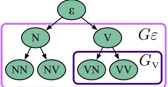
Figure 2: A visual depiction of the tree-structured group lasso penalty. Each node represents a tag string feature. The group indexed by a node’s tag string is defined as the
setof features that areproper descendantsof the node. For example, thelavenderbox indicates the largest group Gεand theauberginebox indicates a smaller groupGV. To avoid clutter, not all groups are marked.
ofWunder prefixes and last-character replacement. (Any tag strings in W\W can get nonzero weight
without increasing runtime.) Thus,R(θ)would
ide-ally measure|W|, or proportionately,|H|. Experi-mentally, we find that|W|has>99%Pearson
cor-relation with wallclock time, making it an excellent proxy for wallclock time while being more replicable.
We relax this regularizer to a convex function— a tree-structured group lasso objective (Yuan and Lin, 2006; Nelakanti et al., 2013). For each string
h ∈ Y∗, we have a groupGhconsisting of the
in-dicator features (inf(2)) for all stringsw∈ Wthat
havehas a proper prefix. Fig. 2 gives a visual depic-tion. We now defineR(θ) =Ph∈Y∗||θGh||2. This
penalty encourages each group of weights to remain all at zero (thereby conserving runtime, in our setting, because it means thathdoes not need to be added
to H). Once a single weight in a group becomes
nonzero, the “initial inertia” induced by the group lasso penalty is overcome, and other features in the group can be more cheaply adjusted away from zero.
Although eq. (1) is now convex, directly optimiz-ing it would be expensive for largek, sinceθthen
contains very many parameters. We thus use a heuris-tic optimization algorithm, the active set method (Schmidt, 2010), which starts with a low-dimensional
θandincrementallyadds features to the model. This
also frees us from needing to specify a limitk. Rather,
Wgrows until further extensions are unhelpful, and
then implicitlyk= maxw∈W|w| −1.
active set iteration, we fully optimize eq. (1) to obtain a sparseθand a setW ={w∈ Wactive |θ(2)w 6= 0}
of features that are known to be “useful.”5We then update Wactive to{wy | w ∈ W, y ∈ Y}, so that it includes single-tag extensions of these useful fea-tures; this expandsθto consider additional features
that plausibly might prove useful. Finally, we com-plete the iteration by updatingWactive to its closure
Wactive, simply because this further expansion of the feature set will not slow down our algorithms. When eq. (1) is re-optimized at the next iteration, some of these newly added features in Wactive may acquire nonzero weights and thus enterW, allowing further
extensions. We can halt onceW no longer changes. As a final step, we follow common practice by running “debiasing” (Martins et al., 2011a), where we fix ourf(2)feature set to be given by the finalW,
and retrainθwithout the group lasso penalty term.
In practice, we optimized eq. (1) using the online proximal gradient algorithm SPOM(Martins et al., 2011b) and Adagrad (Duchi et al., 2011) withη = 0.01and15inner epochs. We limited to3active set
iterations, and as a result, our finalW contained at most tag trigrams.
4 Related Work
Our paper can be seen as transferring methods of Cotterell and Eisner (2015) to the CRF setting. They too used tree-structured group lasso and active set to select variable-ordern-gram featuresW for
globally-normalized sequence models (in their case, to rapidly and accurately approximate beliefs during message-passing inference). Similarly, Nelakanti et al. (2013) used tree-structured group lasso to regu-larize a variable-order language model (though their focus wastrainingspeed). Here we apply these tech-niques toconditionalmodels for tagging.
Our work directly builds on the variable-order CRF of Cuong et al. (2014), with a speedup in Alg. 2, but our approach also learns the VoCRF structure. Our method is also related to thegenerativevariable-order tagger of Sch¨utze and Singer (1994).
Our static feature selection chooses a single model that permits fast exact marginal inference, similar to learning a low-treewidth graphical model (Bach and
5Each gradient computation in this inner optimization takes time O(|Wactive|n), which is especially fast at early iterations.
Jordan, 2001; Elidan and Gould, 2008). This con-trasts with recent papers that learn to do approximate
1-best inference using a sequence of models, whether
by dynamic feature selection within a greedy infer-ence algorithm (Strubell et al., 2015), or by gradually increasing the feature set of a1-best global inference
algorithm and pruning its hypothesis space after each increase (Weiss and Taskar, 2010; He et al., 2013).
Schmidt (2010) explores the use of group lasso penalties and the active set method for learning the structure of a graphical model, but does not consider learning repeated structures (in our setting,
Wdefines a structure that is reused at each position). Steinhardt and Liang (2015) jointly modeled the amount of context to use in a variable-order model that dynamically determines how much context to use in a beam search decoder.
5 Experiments6
Data:We conduct experiments on multilingual POS tagging. The task is to label each word in a sen-tence with one of|Y|= 17labels. We train on five
typologically-diverse languages from the Universal Dependencies (UD) corpora (Petrov et al., 2012): Basque, Bulgarian, Hindi, Norwegian and Slovenian. For each language, we start with the original train / dev / test split in the UD dataset, then move random sentences from train into dev until the dev set has
3000sentences. This ensures more stable
hyperpa-rameter tuning. We use these new splits below. Eval: We train models with (λ, γ) ∈ {10−4 ·
m,10−3·m,10−2·m}×{0,0.1·m,0.2·m, . . . , m},
wheremis the number of training sentences. To tag
a dev or test sentence, we choose its most probable tag sequence. For each of several model sizes, Ta-ble 1 selects the model of that size that achieved the highest per-token tagging accuracy on the dev set, and reports that model’s accuracy on the test set.
Features:Recall from§3 that our features include
non-stationary zeroth-order featuresf(1)as well as
the stationary features based onW. Forf(1)(x, t, yt)
we consider the following language-agnostic proper-ties of(x, t):
• The identities of the tokens xt−3, ..., xt+3,
and the token bigrams (xt+1, xt), (xt, xt−1), 6Code and data are available at the following URLs:
k-CRF (|W|= 17k+1) VoCRF at different model sizes
|W|(which is proportional to runtime)
0 (17) 1 (289) 2 (4913) ≤34 ≤85 ≤170 ≤340 ≤850 ≤1700 ≤2550 ≤3400 ≤4250 ≤5100
Ba 91.611,292.350 92.490 92.250,2 92.250,2 92.380 92.340 92.440 92.440 92.440 92.540 92.540 92.540
Bu 96.481,297.110,297.290,196.750,1,296.780,1,296.990,1,297.080,297.180,197.250,1 97.340,197.340,197.340,197.340,1
Hi 95.961,296.220 96.210 95.971,2 96.220 96.220 96.260 96.130 96.130 96.240 96.240 96.240 96.240
No 96.001,296.640 96.660 96.071,2 96.260,1,296.410 96.600 96.620 96.640 96.670 96.640 96.640 96.640
Sl 94.461,295.410,295.620,194.821,2 95.180,2 95.360,2 95.390,295.390,295.690,195.690,1 95.690,195.690,195.670,1 Table 1: Part-of-speech tagging with Universal Tags: This table shows test results on5languages at different target runtimes. Each row’s best results are inboldface, where ties in accuracy are broken in favor of faster models. Superscript kindicates that the accuracy is significantly different from thek-CRF (paired permutation test,p < 0.05) and this superscript is inblue/redif the accuracy is higher/lower than thek-CRF. In all cases, we find a VoCRF (underlined) that is about as accurate as the2-CRF (i.e., not significantly less accurate) and far faster, since the2-CRF has|W|= 4913. Fig. 1 plots the Pareto frontiers.
(xt−1, xt+1). We use special boundary symbols
for tokens at positions beyond the start or end of the sentence.
• Prefixes and suffixes ofxt, up to4 characters
long, that occur≥5times in the training data.
• Indicators for whether xt is all caps, is
lowercase, or has a digit.
• Word shape ofxt, which maps the token string
into the following character classes (uppercase, lowercase, number) with punctuation unmod-ified (e.g.,VoCRF-like⇒AaAAA-aaaa,$5,432.10 ⇒$8,888.88).
For efficiency, we hash these properties into222bins.
Thef(1) features are obtained by conjoining these
bins withyt(Weinberger et al., 2009): e.g., there is
a feature that returns 0 unlessyt=NOUN, in which
case it counts the number of bin 1234567’s properties that(x, t)has. (Thef(2) features are not hashed.)
Results: Our results are presented in Fig. 1 and Table 1. We highlight two key points: (i) Acrossall languageswe learned a tagger about as accurate as a 2-CRF, but much faster. (ii) The size of the set
W required is highly language-dependent. For many languages, learning a full k-CRF is wasteful; our
method resolves this problem.
In each language, the fastest “good” VoCRF is rather faster than the fastest “good”k-CRF (where
“good” means statistically indistinguishable from the 2-CRF). These two systems are underlined; the un-derlined VoCRF systems are smaller than the under-lined k-CRF systems (for the 5 languages respec-tively) by factors of1.9, 6.4, 3.4, 1.9, and2.9. In
every language, we learn a VoCRF with|W| ≤850
that is not significantly worse than a 2-CRF with
|W|= 173= 4913.
We also notice an interesting language-dependent effect, whereby certain languages require a small number of tag strings in order to perform well. For example, Hindi has a competitive model that ignores the previous tag yt−1 unless it is in
{NOUN,VERB,ADP,PROPN}: thus the stationary fea-tures are 17 unigrams plus4×17bigrams, for a total
of|W| = 85. At the other extreme, the Slavic
lan-guages Slovenian and Bulgarian seem to require more expressive models over the tag space, remembering as many as 98 useful left-context histories (unigrams and bigrams) for the current tag. An interesting direc-tion for future research would be to determine which morpho-syntactic properties of a language tend to increase the complexity of tagging.
6 Conclusion
We presented a structured sparsity approach for struc-ture learning in VoCRFs, which achieves the accu-racy of higher-order CRFs at a fraction of the runtime. Additionally, we derive an asymptotically faster al-gorithm for the gradients necessary to train a VoCRF than prior work. Our method provides an effective speed-accuracy tradeoff for POS tagging across five languages—confirming that significant speed-ups are possible with little-to-no loss in accuracy.
References
Cyril Allauzen, Mehryar Mohri, and Brian Roark. 2003. Generalized algorithms for constructing statistical lan-guage models. InProceedings of ACL, pages 40–47. F. R. Bach and M. I. Jordan. 2001. Thin junction trees. In
NIPS, pages 569–576.
Ryan Cotterell and Jason Eisner. 2015. Penalized expec-tation propagation for graphical models over strings. In
NAACL-HLT, pages 932–942.
Nguyen Viet Cuong, Nan Ye, Wee Sun Lee, and Hai Leong Chieu. 2014. Conditional random field with high-order dependencies for sequence labeling and segmentation.
JMLR, 15(1):981–1009.
John Duchi, Elad Hazan, and Yoram Singer. 2011. Adaptive subgradient methods for online learning and stochastic optimization. JMLR, 12:2121–2159. Jason Eisner. 2016. Inside-outside and forward-backward
algorithms are just backprop. InProceedings of the EMNLP 16 Workshop on Structured Prediction for NLP, Austin, TX, November.
G. Elidan and S. Gould. 2008. Learning bounded treewidth Bayesian networks. InNIPS, pages 417–424. He He, Hal Daum´e III, and Jason Eisner. 2013. Dynamic
feature selection for dependency parsing. InEMNLP, pages 1455–1464.
John D. Lafferty, Andrew McCallum, and Fernando C. N. Pereira. 2001. Conditional random fields: Probabilistic models for segmenting and labeling sequence data. In
ICML, pages 282–289.
Percy Liang, Hal Daum´e III, and Dan Klein. 2008. Struc-ture compilation: trading strucStruc-ture for feaStruc-tures. In
ICML, pages 592–599.
Andr´e F. T. Martins, Noah A. Smith, Pedro M. Q. Aguiar, and M´ario A. T. Figueiredo. 2011a. Structured sparsity in structured prediction. InEMNLP, pages 1500–1511. Andr´e F. T. Martins, Noah A. Smith, Eric P. Xing, Pe-dro M. Q. Aguiar, and M´ario A.T. Figueiredo. 2011b. Online learning of structured predictors with multiple kernels. InAISTATS, pages 507–515.
Anil Nelakanti, Cedric Archambeau, Julien Mairal, Fran-cis Bach, and Guillaume Bouchard. 2013. Structured penalties for log-linear language models. InEMNLP, pages 233–243.
Slav Petrov, Dipanjan Das, and Ryan T. McDonald. 2012. A universal part-of-speech tagset. InLREC, pages 2089–2096.
Mark Schmidt. 2010.Graphical Model Structure Learn-ing with`1-Regularization. Ph.D. thesis, University of
British Columbias.
Hinrich Sch¨utze and Yoram Singer. 1994. Part-of-speech tagging using a variable memory Markov model. In
ACL, pages 181–187.
Jacob Steinhardt and Percy Liang. 2015. Reified context models. InICML, pages 1043–1052.
Emma Strubell, Luke Vilnis, Kate Silverstein, and Andrew McCallum. 2015. Learning dynamic feature selection for fast sequential prediction. InACL, pages 146–155. Kristina Toutanova, Dan Klein, Christopher D. Manning, and Yoram Singer. 2003. Feature-rich part-of-speech tagging with a cyclic dependency network. In ACL, pages 173–180.
Kilian Weinberger, Anirban Dasgupta, John Langford, Alex Smola, and Josh Attenberg. 2009. Feature hash-ing for large scale multitask learnhash-ing.
David J. Weiss and Benjamin Taskar. 2010. Structured prediction cascades. InAISTATS, pages 916–923. Nan Ye, Wee S. Lee, Hai L. Chieu, and Dan Wu. 2009.
Conditional random fields with high-order features for sequence labeling. InNIPS, pages 2196–2204. Ming Yuan and Yi Lin. 2006. Model selection and