HMM Specialization with Selective Lexicalization

(1)

I

H M M S p e c i a l i z a t i o n w i t h Selective Lexicalization*

J i n - D o n g K i m a n d S a n g - Z o o L e e a n d H a e - C h a n g R i m Dept. of C o m p u t e r Science a n d Engineering, K o r e a University,

A n a m - d o n g , S e o n g b u k - k u , Seoul 136-701, K o r e a E - m a i h {jinlzoolrim}@nlp.korea.ac.kr

A b s t r a c t

We present a technique which complements Hidden Markov Models by incorporating some lexicalized states representing syntactically uncommon words. ' O u r approach examines the distribution of transitions, selects the uncommon words, and makes lexicalized states for the words. We perfor'med a part-of-speech tagging experiment on the Brown corpus to evaluate the resultant language model and discovered that this technique improved the tagging accuracy by 0.21% at the 95% level of confidence.

1 I n t r o d u c t i o n

Hidden Markov 'Models are widely used for statistical language modelling in various fields, e.g., part-of-speech tagging or speech recogni- tion (Rabiner and Juang, 1986). The models are based on Markov assumptions, which make it possible to view the language prediction as a Markov process. 'In general, we make the first- order Markov ass'umptions that the current tag is only dependant on the previous tag and that the current word is only dependant on the current tag. These are very 'strong' assumptions, so that the first-order Hidden Markov Models have the advantage of drastically reducing the number of its parameters. On the other hand, the assumptions restrict the model from utiliz- ing enough constraints provided by the local context and the resultant model consults only a single category 'as the contex.

A lot of effort has been devoted in the past to make up for the insufficient contextual information of the first-order probabilistic model. The second order Hidden Markov Models with

" T h e research u n d e r l y i n g this p a p e r was s u p p o r t e d t) 3" research g r a n t s fl'om K o r e a Science a n d E n g i n e e r i n g F o u n d a t i o n .

appropriate smoothing techniques show better performance than the first order models and is considered a state-of-the-art technique (Meri- aldo, 1994; Brants, 1996). The complexity of the model is however relatively very high considering the small improvement of the performance.

Garside describes IDIOMTAG (Garside et al., 1987) which is a component of a part-of- speech tagging system named CLAWS. ID- IOMTAG serves as a front-end to the tagger and modifies some initially assigned tags in order to reduce the amount of ambiguity to be dealt with by the tagger. IDIOMTAG can look at any combination of words and tags, with or without intervening words. By using the IDIOMTAG, CLAWS system improved tagging accuracy from 94% to 96-97%. However, the manual-intensive process of producing id- iom tags is very expensive although IDIOMTAG proved fruitful.

Kupiec (Kupiec, 1992) describes a technique of augmenting the Hidden Markov Models for part-of-speech tagging by the use of networks. Besides the original states representing each part-of-speech, the network contains additional states to reduce the noun/adjective confusion, and to extend the context for predicting past participles from preceding auxiliary verbs when they are separated by adverbs. By using these additional states, the tagging system improved the accuracy from 95.7% to 96.0%. However, the additional context is chosen by analyzing the tagging errors manually.

(2)

new states represents a extended context. With this technique, Brants reported a performance cquivalent to the second order Hidden Markov Models.

In this paper, we present an automatic re- fining technique for statistical language models. First, we examine the distribution of transitions of lexicalized categories. Next, we break out the u n c o m m o n ones from their categories and make new states for them. All processes are auto- m a t e d and the user has only to determine the extent of the breaking-out.

2 " S t a n d a r d " P a r t - o f - S p e e c h T a g g i n g M o d e l b a s e d o n H M M

From the statistical point of view, the tagging problem can be defined as the problem of find- ing the proper sequence of categories c:,r~ = Cl, c2, ..., cn (n _> 1) given the sequence of words

w:,n = wl, w2, ...,wn (We denote the i'th word by wi, and the category assigned to the wi by

ci), which is formally defined by the following equation:

"]-(Wl,n) -= argmaxP(Cl,nlW:,~) (1)

Charniak (Charniak et al., 1993) describes the "standard" HMM-based tagging model as Equation 2, which is the simplified version of Equation 1.

n

T(w:,~)

= arg max I I P(cilci-1)P(wilci) (2)

i n . ' z - - - - I

W i t h this model, we select the proper category for each word by making use of the contextual probabilities, P(citci_ 1), and the lexical probabilities, P(wilci). This model has the advan- tages of a provided theoretical framework, automatic learning facility and relatively high performance. It is thereby at the basis of most tagging programs created over the last few years.

For this model, the first-order Markov assum- tions are m a d e as follows:

P(cilcl,i-l,Wl,i_l) ~ P(cilci-1) (3)

P(wi[cd

(4)

W i t h Equation 3, we assume that the current category is independent of the previous words and only dependent on the previous category.

With Equation 4, we also assume that the correct word is independent of everything except the knowledge of its category. T h r o u g h these assmnptions, the Hidden Markov Models have the advantage of drastically reducing the number of parameters, thereby alleviating the sparse d a t a problem. However, as mentioned above, this model consults only a single category as context and does not utilize enough constraints provided by the local context.

3 S o m e R e f i n i n g T e c h n i q u e s f o r H M M

Tile first-order Hidden Markov Models de- scribed in the previous section provides only a single category as context. Sometimes, this first-order context is sufficient to predict the following parts-of-speech, but at other times (probably much more often) it is insufficient. The goal of the work reported here is to develop a m e t h o d that can automatically refine the Hid- den Markov Models to produce a more accu- rate language model. We start with the care- ful observation on the assumptions which are made for the "standard" Hidden Markov Mod- els. W i t h the Equation 3, we assume t h a t the current category is only d e p e n d e n t on the preceding category. As we know, it is not always true and this first-order Markov assumption re- stricts the disambiguation information witlfin the first-order context.

T h e immediate ways of enriching the context are as follows:

• to lexicalize the context.

• to extend the context to higher-order.

To lexiealize the context, we include the preceding word into the context. Contextual probabilities are then defined by

P(eilci_l,Wi-1).

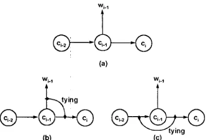
Figure 1 illustrates the change of d e p e n d e n c y when each m e t h o d is applied respectively. Fig- ure l(a) represents that each first-order contextual probability and lexical probability are in- d e p e n d e n t of each other in the "standard" Hid- den Markov Models, where Figure l(b) represents t h a t the lexical probability of the preceding word and the contextual probability of the current category are tied into a lexicalized contextual probability.

(3)

Wi.1

(a)

Wi., I Wi.t

(b) (c)

Figure 1: Two T y p e s of Weakening the Markov Assumption

order. Contextual probabilities are then defined by

P(cilci_l,Ci_2).

Figure l(c) represents that the two adjacent contextual probabilities are tied into the sec0nd-order contextual probability.

The simple way of enriching the context is to extend or lexica!ize it uniformly. The uniform extension of context to the second order is fea- sible with an appropriate smoothing technique and is considered a state-of-the-art technique, though its complexity is very high: In the case of the Brown cerpus, we need trigrams up to the number of 0.6 million. An alternative to the uniform extension of context is the selective extension of c o n t e x t . Brants(Brants, 1996) takes this approach and reports a performance equiv- alent to the uniform extension with relatively much low complexity of the model.

The uniform lexicalization of context is com- putationally prohibitively expensive: In the case of the Brown corpus, we need lexicalized bigrams up to the number of almost 3 billion. Moreover, m a n y l o f these bigrams neither con- tribute to the per~formance of the model, nor oc- cur frequently enough to be estimated properly. An alternative to the uniform lexicalization is the selective lexicalization of context, which is the main topic of this paper.

4 S e l e c t i v e L e x i c a l i z a t i o n o f H M M

This section describes a new technique for re- fining the Hidden Markov Model, which we call selective lexicalization. Our approach automatically finds out s'yntactically uncommon words and makes a new state (we call it a l e x i e a l i z e d

s t a t e ) f o r each of the words.

Given a fixed set of categories, {C 1 , C 2, ...,

cC},

e.g.,

{adjective,..., verb},

we assume the dis- crete r a n d o m variable XcJ with domain the set of categories and range a set of conditional probabilities. The r a n d o m variable XcJ then represents a process of assigning a conditional probability

p(cilc j)

to every category

c i

(e i ranges

over

cl ...c C)

xc (c = P ( d

= P ( c 2 1 c J )

Xc) (c C) = p(cClc j)

We convert the process of

Xcj

into the s t a t e t r a n s i t i o n v e c t o r , VcJ , which consists of the corresponding conditional probabilities, e.g.,

Vprep

- - - -

( P(adjectiveiprep), ..., P(verbiprep) ) T.

The (squared) distance between two arbitrary vectors is then c o m p u t e d as follows:

l ~ ( V l , V 2 ) = ( V l -- v 2 ) T ( v 1 - V 2 ) (5)

Similarly, we define the l e x i c a l i z e d s t a t e t r a n s i t i o n v e c t o r 1, VO,wk , e.g.,

V p r e p , i n -~

( P (adjectivelprep,

in),...,

P (verblprep, in)) Y

In this situation, it is possible to regard each lexicMized state transition vector, VcJ,wk, of the same category cJ as members of a cluster whose centroid is the state transition vector, Vc). We can then c o m p u t e the deviation of each lexicalized state transition vector, Vc~,wk , from its corresponding centroid.

T

D(Vc¢,wk ) = ( V c ~ , ~ k - V d )

(VcJ,wJ-Vcj)

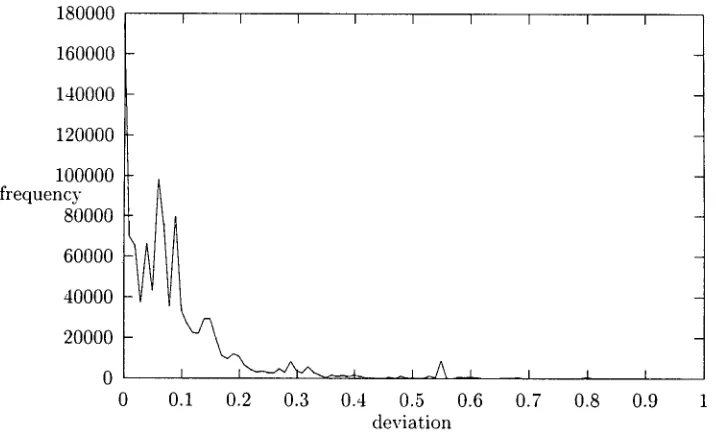
(6)

Figure 2 represents the distribution of lexicalized state transition vectors according to their deviations. As you can see in the figure, the majority of the vectors are near their centroids and only a small number of vectors are very far from their centroids. In the first-order context model (without considering lexicalized context).

[image:3.612.71.283.72.216.2]

(4)

180000

160000

140000

120000

100000 ~equency

80000

60000

40000

20000

0

f I I I I I I I I

0.1 0.2 0.3 0.4

A i ~ • _ 1 1 I

0 0.5 0.6 0.7 0.8 0.9 1

deviation

Figure 2: Distribution of Lexicalized Vectors according to Deviation

the centroids represent all the members belong- ing to it. In fact, the deviation of a vector is a kind of (squared) error for the vector. The error for a cluster is

e(VcJ)

= ~ D(Vd,wk ) (7)

W k

and the error for the overall model is simply the sum of the individual cluster errors:

E = ~ e ( V g ) (8) cJ

Now, we could break out a few lexicalized state vectors which have large deviation (D > 0) and make t h e m individual clusters to reduce the error of the given model.

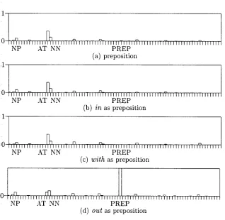
As an example, let's consider the p r e p o s i - t i o n cluster. The value of each component of the centroid,

Vprep,

is illustrated in Figure 3(a) and that of the lexicalized vectors,

Vprep,in,

Vprep,wit h and Vprep,out a r e in Figure 3(b), (c)

and (d) respectively. As you can see in these figures, most of the prepositions including

in

and

with

are immediately followed by article(AT), noun(NN) or pronoun(NP), but the word

out

as preposition shows a completely different distribution. Therefore, it would be a good choice to break out the lexicalized vector, Vprep,out , froln its centroid, Vprep.

o u t

a t * - - w i t h

(a) (b)

Figure 4: Splitting the p r e p o s i t i o n State

From the viewpoint of a network, the state representing p r e p o s i t i o n is split into two states; the one is the state representing ordi- nary prepositions except

out,

and the other is the state representing the special preposition

out,

which we call a l e x i c a l i z e d s t a t e . This process of splitting is illustrated in Figure 4.

Splitting a state results in some changes of the parameters. T h e changes of the parameters resulting from lexicalizing a word,

w k,

in a category, C j, a r e indicated in Table 1

(c i

ranges

over

cl...cC).

This full splitting will increase the complexity of the model rapidly, so that estimating the p a r a m e t e r s m a y suffer from the sparseness of the data.

[image:4.612.129.487.59.276.2] [image:4.612.332.546.331.443.2]

(5)

1

I I I I I I l I T I II1~1111111111~11 11111~11111171111111111 I I I T I I I I T I I ~ I I I I I I I

NP AT NN PREP

(a) preposition

0 ,~llri71 I,l,llll,ll-rll?ll , , , l l , l l l l l l l , i i i l i T i l i l iliT, ii II,illll

NP AT NN PREP

(b)

in

as preposition

1

!

~0 JN, IiITI IIItl,,llliT,IrT'llllll~,,~ll~ll,llllllTIl,I li~Tllt ItT~tttt

NP AT NN PREP

(c)

with

as preposition

NP AT NN PREP

(d)

out

as preposition

Figure 3: Transition Vectors in p r e p o s i t i o n Cluster

Table 1: Changes of Parameters in Full Split- ting

before splitting after splitting

P(w~lc y)

P(cil~)

P ( d l c i )

p(wilcJ, w k) p ( w i l c j , ~W k)

P(dlcJ , w k)

P(cilcJ, ~w k)

P(cJ, w k Ic i)

P(cJ, -~w~l ci)

parameters. The changes of the parameters in pseudo splitting ate indicated in Table 2.

5 E x p e r i m e n t a l R e s u l t

We have tested our technique through part-of- speech tagging eXperiments with the Hidden Markov Models which are variously lexicalized. In ordcr to conduct the tagging experiments, we divided the whole Brown (tagged) corpus containing 53,887 sentences (1,113,191 words) into two parts. For tlle t r a i n i n g set. 90% of the

Table 2: Changes of P a r a m e t e r s in Pseudo Splitting

before splitting after splitting

P ( w ' l d )

P(w~l d)

P(cilc j)

p(cilcJ, w k)

p(cilc j, ~w k)

P(elc

P(c lc')

sentences were chosen at random, from which we collected all of the statistical data. We re- served the other 10% for testing. Table 3 lists the basic statistics of our corpus.

Table 3: Overview of Our Corpora

I # of sentences # of words training set 48,499 1,001,712

[image:5.612.142.460.59.369.2] [image:5.612.88.253.455.555.2] [image:5.612.321.494.455.528.2]

(6)

We used a tag set containing 85 categories. The amount of ambiguity of the test set is sum- marized in Table 4. The second column shows that words to the ratio of 52% (the number of 57,808) are not ambiguous. The tagger at- tempts to resolve the ambiguity of the remain- ing words.

Table 4: Amount of Ambiguity of Test Set

I a m b i g u i t y ( # ) 3 4

ratio(%) 5 1 2 1 : 0 1 8 71 5 1 I total ₁₀₀

I

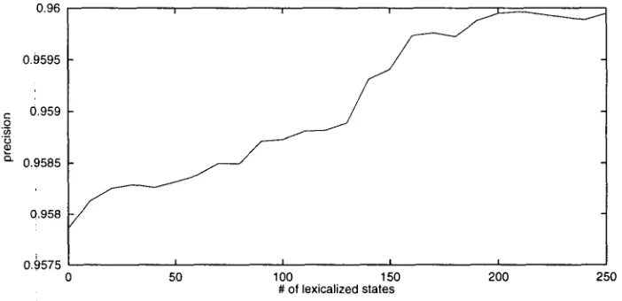
Figure 5 and Figure 6 show the results of our part-of-speech tagging experiments with the "standard" Hidden Markov Model and variously lexicalized Hidden Markov Models using full splitting method and pseudo splitting m e t h o d respectively.

We got 95.7858% of the tags correct when we applied the standard Hidden Markov Model without any lexicalized states. As the number of lexicalized states increases, the tagging accuracy increases until the number of lexicalized states becomes 160 (using full splitting) and 210 (using pseudo splitting). As you can see in these figures, the full splitting improves the performance of the model more rapidly but suffer more sevelery from the sparseness of the training data. In this experiment, we employed Mackay and Peto's smoothing techniques for estimating the parameters required for the models. The best precision has been found to be 95:9966% through the model with the 210 lexcalized states using the pseudo splitting method.

6 C o n c l u s i o n

In this paper, we present a m e t h o d for comple- menting the Hidden Markov Models. With this method, we lexicalize the Hidden Markov Model seletively and automatically by examining the transition distribution of each state relating to certain words.

Experimental results showed that the selective lexicalization improved the tagging accu- rary from about 95.79% to about 96.00%. Using normal tests for statistical significance we found that the improvement is significant at the 95% level of confidence.

Tile cost for this imt~rovenmnt is minimal. The resulting network contains 210 additional lexicalized states which are found automatically. Moreover, the lexicalization will not de- crease the tagging speed 2, because the lexicalized states and their corresponding original states are exclusive in our lexicalized network, and thus the rate of ambiguity is not increased even if the lexicalized states are included.

Our approach leaves much room for improvement. We have so far considered only the outgo- ing transitions from the target states. As a re- sult, we have discriminated only the words with right-associativity. We could also discriminate the words with left-associativity by examining the incoming transitions to the state. Further- more, we could extend the context by using the second-order context as represented in Figure l(c). We believe that the same technique pre- sented in this paper could be applied to the pro- posed extensions.

R e f e r e n c e s

T. Brants. 1996. Estimating markov model structures. In Proceedings of the Fourth In- ternational Conference on Spoken Language

Processing, pages 893-896.

E. Charniak, C. Hendrickson, N. Jacobson, and M. Perkowitz. 1993. Equations for part-of-speech tagging. In Proceedings of the Eleventh National Conference on Artificial Intelligence, pages 784-789.

K. Church. 1988. A stochastic parts program and noun phrase parser for unrestricted text.

In Proceedings of the Second Conference on

Applied Natural Language Processing, pages

136-143.

S. Derose. 1988. Grammatical category disambiguation by statistical optimization. Com- putational Linguistics, 14(1):31-39.

R. Garside, G. Leech, and G. Sampson. 1987. The Computational Analysis of En-

glish. Longman Group.

J. Kupiec. 1992. Robust part-of-speech tagging using a hidden markoV model. Computer

Speech and Language, 6:225-242.

D. MacKay and L. Peto. 1995. A hierarchical dirichlet language model. Natural Language

Engineering, 1(3):289-307.

(7)

i

I

0.96

0.9595

.~

0.959

0.9585

0.958

0.9575 I I I I

50 100 150 200 250

# of lexicalized states

Figure 5: POS tagging results with lexicalized HMM using full splitting method

0.96

0.9595

0.959

Q" 0.9585

0.958

f

|

0.9575 I I I I

0 50 100 150 200

# oflexicalized states

250

Figure 6: POS tagging results with lexicalized HMM using pseudo splitting method

B. Merialdo. 1994. Tagging english text with a

probabilistic model.

Computational Linguis-

tics,

20(4):155-171.

L. Rabiner and B. Juang. 1986. An introduc-

tion to hiddeii markov models.

IEEE ASSP

Magazine,

pages 4-16, January.

A p p e n d i x :

Top 100 words w i t h high deviation

according(IN) l"ather(IN) out(IN) able(J J)

Aj(NP) no(QL) because(RB) however(RB)

as(IN) per(IN) trying(VBG) however(WRB)

likely(J J) Uuited(NP) Mrs.(NP) New(NP)

Rhode(NP)

. National(NP)

Miss(NP)

tried(VBD)

Dr)(NP)

lack(NN) nmch(QL)

Mr.(NP)

North(NP)

June(NP)

A.(NP)

J.(NP)

right(QL)

May(NP)

ready(J J)

St.(NP)

even(QL)

various(J J) don't(DO)

instead(RB) far(QL) B(NP) didn't(DOD)

try(VB) available(JJ) William(NP)!(.)

?(.)

;(.) number(NN) so(CS) due(J J) World(NP)

Christian(NP)

difficult (J J)

tell(VB)

go-

ing(VBG) kind(NN) let(VB) continue(VB)

series(NN)

part(NN)

radio(NN)

sure(J J)

want(VB) front(NN) seem(VB) total(NN)

decided(VBD)

expected(VBN)

right(NN)

based(VBN) White(NP) except(IN) told(VBD)

James(NP) fact(NN) March(NP) sort(NN)

example(NN)

designed(VBN)

respect(NN)

talk(VB) Department(NP) single(AP) Ne-

gro(NP) wanted(VBD) Western(NP) yes(RB)

become(VBN)

necessary(J J)

speak(VB)

about(RB) amount(NN) down(IN)like(VB)

S.(NP)

same(AP)

too(RB)

General(NP)

[image:7.612.123.469.73.243.2] [image:7.612.123.474.276.446.2]