Two Languages are Better than One (for Syntactic Parsing)

Two Languages are Better than One (for Syntactic Parsing)

David Burkett and Dan Klein Computer Science Division University of California, Berkeley {dburkett,klein}@cs.berkeley.edu

Abstract

We show that jointly parsing a bitext can sub-stantially improve parse quality on both sides. In a maximum entropy bitext parsing model, we define a distribution over source trees, tar-get trees, and node-to-node alignments

be-tween them. Features include monolingual

parse scores and various measures of syntac-tic divergence. Using the translated portion of the Chinese treebank, our model is trained iteratively to maximize the marginal likeli-hood of training tree pairs, with alignments treated as latent variables. The resulting bi-text parser outperforms state-of-the-art mono-lingual parser baselines by 2.5 F1at predicting

English side trees and 1.8 F1at predicting

Chi-nese side trees (the highest published numbers on these corpora). Moreover, these improved trees yield a 2.4 BLEU increase when used in a downstream MT evaluation.

1 Introduction

Methods for machine translation (MT) have increas-ingly leveraged not only the formal machinery of syntax (Wu, 1997; Chiang, 2007; Zhang et al., 2008), but also linguistic tree structures of either the source side (Huang et al., 2006; Marton and Resnik, 2008; Quirk et al., 2005), the target side (Yamada and Knight, 2001; Galley et al., 2004; Zollmann et al., 2006; Shen et al., 2008), or both (Och et al., 2003; Aue et al., 2004; Ding and Palmer, 2005). These methods all rely on automatic parsing of one or both sides of input bitexts and are therefore im-pacted by parser quality. Unfortunately, parsing gen-eral bitexts well can be a challenge for newswire-trained treebank parsers for many reasons, including out-of-domain input and tokenization issues.

On the other hand, the presence of translation pairs offers a new source of information: bilin-gual constraints. For example, Figure 1 shows a case where a state-of-the-art English parser (Petrov and Klein, 2007) has chosen an incorrect structure which is incompatible with the (correctly chosen) output of a comparable Chinese parser. Smith and Smith (2004) previously showed that such bilin-gual constraints can be leveraged to transfer parse quality from a rich language to a resource-impoverished one. In this paper, we show that bilin-gual constraints and reinforcement can be leveraged to substantially improve parses on both sides of a bitext, even for two resource-rich languages.

Formally, we present a log-linear model over triples of source trees, target trees, and node-to-node tree alignments between them. We consider a set of core features which capture the scores of monolingual parsers as well as measures of syntactic alignment. Our model conditions on the input sen-tence pair and so features can and do reference input characteristics such as posterior distributions from a word-level aligner (Liang et al., 2006; DeNero and Klein, 2007).

Our training data is the translated section of the Chinese treebank (Xue et al., 2002; Bies et al., 2007), so at training time correct trees are observed on both the source and target side. Gold tree align-ments are not present and so are induced as latent variables using an iterative training procedure. To make the process efficient and modular to existing monolingual parsers, we introduce several approxi-mations: use ofk-best lists in candidate generation, an adaptive bound to avoid considering allk2 com-binations, and Viterbi approximations to alignment posteriors.

Figure 1: Two possible parse pairs for a Chinese-English sentence pair. The parses in a) are chosen by independent monolingual statistical parsers, but only the Chinese side is correct. The gold English parse shown in b) is further down in the 100-best list, despite being more consistent with the gold Chinese parse. The circles show where the two parses differ. Note that in b), the ADVP and PP nodes correspond nicely to Chinese tree nodes, whereas the correspondence for nodes in a), particularly the SBAR node, is less clear.

We evaluate our system primarily as a parser and secondarily as a component in a machine translation pipeline. For both English and Chinese, we begin with the state-of-the-art parsers presented in Petrov and Klein (2007) as a baseline. Joint parse selection improves the English trees by 2.5 F1 and the Chi-nese trees by 1.8 F1. While other Chinese treebank parsers do not have access to English side transla-tions, this Chinese figure does outperform all pub-lished monolingual Chinese treebank results on an equivalent split of the data.

As MT motivates this work, another valuable evaluation is the effect of joint selection on down-stream MT quality. In an experiment using a syntactic MT system, we find that rules extracted from joint parses results in an increase of 2.4 BLEU points over rules extracted from independent parses.1 In sum, jointly parsing bitexts improves parses substantially, and does so in a way that that carries all the way through the MT pipeline.

2 Model

In our model, we consider pairs of sentences(s, s0), where we use the convention that unprimed vari-ables are source domain and primed varivari-ables are target domain. These sentences have parse trees t (respectively t0) taken from candidate sets T (T0).

1

It is anticipated that in some applications, such as tree trans-ducer extraction, the alignments themselves may be of value, but in the present work they are not evaluated.

Non-terminal nodes in trees will be denoted by n (n0) and we abuse notation by equating trees with their node sets. Alignments aare simply at-most-one-to-one matchings between a pair of treestand t0(see Figure 2a for an example). Note that we will also mentionwordalignments in feature definitions; aand the unqualified termalignmentwill always re-fer to node alignments. Words in a sentence are de-noted byv(v0).

Our model is a general log-linear (maximum en-tropy) distribution over triples(t, a, t0)for sentence pairs(s, s0):

P(t, a, t|s, s0)∝exp(w>φ(t, a, t0))

Features are thus defined over (t, a, t0) triples; we discuss specific features below.

3 Features

To use our model, we need features of a triple

(t, a, t0)which encode both the monolingual quality of the trees as well as the quality of the alignment between them. We introduce a variety of features in the next sections.

3.1 Monolingual Features

by our baseline monolingual parsers. These two fea-tures are called SOURCELL and TARGETLL

respec-tively. It is certainly possible to augment these sim-ple features with what would amount to monolin-gual reranking features, but we do not explore that option here. Note that with only these two features, little can be learned: all positive weightswcause the jointly optimal parse pair(t, t0)to comprise the two top-1 monolingual outputs (the baseline).

3.2 Word Alignment Features

All other features in our model reference the entire triple(t, a, t0). In this work, such features are de-fined over aligned node pairs for efficiency, but gen-eralizations are certainly possible.

Bias: The first feature is simply a bias feature which has value 1 on each aligned node pair(n, n0). This bias allows the model to learn a general prefer-ence for denser alignments.

Alignment features: Of course, some alignments are better than others. One indicator of a good node-to-node alignment between nandn0 is that a good word alignment model thinks that there are many word-to-word alignments in their bispan. Similarly, there should be few alignments that violate that bis-pan. To compute such features, we definea(v, v0)

to be the posterior probability assigned to the word alignment betweenvandv0by an independent word aligner.2

Before defining alignment features, we need to define some additional variables. For any noden∈t (n0 ∈ t0), the inside span i(n) (i(n0)) comprises the input tokens of s (s0) dominated by that node. Similarly, the complement, the outside span, will be denotedo(n)(o(n0)), and comprises the tokens not dominated by that node. See Figure 2b,c for exam-ples of the resulting regions.

INSIDEBOTH = X

v∈i(n)

X

v0_∈i(n0₎

a(v, v0)

INSRCOUTTRG =

X

v∈i(n)

X

v0_∈o(n0₎

a(v, v0)

INTRGOUTSRC = X

v∈o(n)

X

v0_∈i(n0₎

a(v, v0)

2_{It is of course possible to learn good alignments using}

lexi-cal indicator functions or other direct techniques, but given our very limited training data, it is advantageous to leverage counts from an unsupervised alignment system.

Hard alignment features: We also define the hard versions of these features, which take counts from the word aligner’s hard top-1 alignment output δ:

HARDINSIDEBOTH = X

v∈i(n)

X

v0_∈i(n0₎

δ(v, v0)

HARDINSRCOUTTRG = X

v∈i(n)

X

v0_∈o(n0₎

δ(v, v0)

HARDINTRGOUTSRC = X

v∈o(n)

X

v0_∈i(n0₎

δ(v, v0)

Scaled alignment features: Finally, undesirable larger bispans can be relatively sparse at the word alignment level, yet still contain many good word alignments simply by virtue of being large. We therefore define a scaled count which measures den-sity rather than totals. The geometric mean of span lengths was a superior measure of bispan “area” than the true area because word-level alignments tend to be broadly one-to-one in our word alignment model.

SCALEDINSIDEBOTH = pINSIDEBOTH

|i(n)| · |i(n0_)|

SCALEDINSRCOUTTRG = _pINSRCOUTTRG

|i(n)| · |o(n0_)|

SCALEDINTRGOUTSRC = pINTRGOUTSRC

|o(n)| · |i(n0)|

Head word alignment features: When consider-ing a node pair(n, n0), especially one which dom-inates a large area, the above measures treat all spanned words as equally important. However, lex-ical heads are generally more representative than other spanned words. Leth select the headword of a node according to standard head percolation rules (Collins, 2003; Bikel and Chiang, 2000).

ALIGNHEADWORD = a(h(n), h(n0))

HARDALIGNHEADWORD = δ(h(n), h(n0))

3.3 Tree Structure Features

We also consider features that measure correspon-dences between the tree structures themselves.

Figure 2: a) An example of a legal alignment on a Chinese-English sentence fragment with one good and one bad node pair, along with sample word alignment posteriors. Hard word alignments are bolded. b) The word alignment regions for the good NP-NP alignment. InsideBoth regions are shaded in black, InSrcOutTrg in light grey, and InTrgOutSrc in grey. c) The word alignment regions for the bad PP-NP alignment.

penalize node pairs whose inside span lengths differ greatly.

SPANDIFF = ||i(n)| − |i(n0)||

Number of children: We also expect that there will be correspondences between the rules of the CFGs that generate the trees in each language. To encode some of this information, we compute in-dicators of the number of childrenc that the nodes have intandt0.

NUMCHILDRENh|c(n)|,|c(n0)|i = 1

Child labels: In addition, we also encode whether certain label pairs occur as children of matched nodes. Letc(n, `)select the children ofnwith la-bel`.

CHILDLABELh`, `0i = |c(n, `)| · |c(n0, `0)|

Note that the corresponding “self labels” feature is not listed because it arises in the next section as a typed variant of the bias feature.

3.4 Typed vs untyped features

For each feature above (except monolingual fea-tures), we create label-specific versions by conjoin-ing the label pair (`(n), `(n0)). We use both the typed and untyped variants of all features.

4 Training

Recall that our data condition supplies sentence pairs(s, s0)along with gold parse pairs(g, g0). We do not observe the alignments a which link these parses. In principle, we want to find weights which maximize the marginal log likelihood of what we do observe given our sentence pairs:3

w∗ = arg max w

X

a

P(g, a, g0|s, s0, w) (1)

= arg max w

P

aexp(w>φ(g, a, g0))

P (t,t0₎

P

aexp(w>φ(t, a, t0))

(2)

There are several challenges. First, the space of symmetric at-most-one-to-one matchings is #P-hard

3

to sum over exactly (Valiant, 1979). Second, even without matchings to worry about, standard meth-ods for maximizing the above formulation would re-quire summation over pairs of trees, and we want to assume a fairly generic interface to independent monolingual parsers (though deeper joint modeling and/or training is of course a potential extension). As we have chosen to operate in a reranking mode over monolingual k-best lists, we have another is-sue: our k-best outputs on the data which trains our model may not include the gold tree pair. We therefore make several approximations and modifi-cations, which we discuss in turn.

4.1 Viterbi Alignments

Because summing over alignmentsais intractable, we cannot evaluate (2) or its derivatives. However, if we restrict the space of possible alignments, then we can make this optimization more feasible. One way to do this is to stipulate in advance that for each tree pair, there is a canonical alignmenta0(t, t0). Of course, we wanta0to reflect actual correspondences betweentandt0, so we want a reasonable definition that ensures the alignments are of reasonable qual-ity. Fortunately, it turns out that we can efficiently optimizeagiven a fixed tree pair and weight vector:

a∗ = arg max

a

P(a|t, t0, s, s0, w)

= arg max

a

P(t, a, t0|s, s0, w)

= arg max

a

exp(w>φ(t, a, t0))

This optimization requires only that we search for an optimal alignment. Because all our features can be factored to individual node pairs, this can be done with the Hungarian algorithm in cubic time.4 Note that we do not enforce any kind of domination con-sistency in the matching: for example, the optimal alignment might in principle have the source root aligning to a target non-root and vice versa.

We then define a0(t, t0) as the alignment that maximizesw₀>φ(t, a, t0), wherew0 is a fixed initial weight vector with a weight of 1 for INSIDEBOTH, -1 for INSRCOUTTRG and INTRGOUTSRC, and 0

4_{There is a minor modification to allow nodes not to match.}

Any alignment link which has negative score is replaced by a zero-score link, and any zero-score link in the solution is con-sidered a pair of unmatched nodes.

for all other features. Then, we simplify (2) by fix-ing the alignmentsa0:

w∗= arg max w

exp(w>φ(g, a0(g, g0), g0)) P

(t,t0₎exp(w>φ(t, a0(t, t0), t0))

(3)

This optimization has no latent variables and is therefore convex and straightforward. However, while we did use this as a rapid training procedure during development, fixing the alignments a priori is both unsatisfying and also less effective than a pro-cedure which allows the alignmentsato adapt dur-ing traindur-ing.

Again, for fixed alignments a, optimizing w is easy. Similarly, with a fixedw, finding the optimal afor any particular tree pair is also easy. Another option is therefore to use an iterative procedure that alternates between choosing optimal alignments for a fixed w, and then reoptimizingw for those fixed alignments according to (3). By iterating, we per-form the following optimization:

w∗= arg max w

maxaexp(w>φ(g, a, g0))

P

(t,t0₎maxaexp(w>φ(t, a, t0))

(4)

Note that (4) is just (2) with summation replaced by maximization. Though we do not know of any guarantees for this EM-like algorithm, in practice it converges after a few iterations given sufficient training data. We initialize the procedure by setting w0as defined above.

4.2 Pseudo-gold Trees

When training our model, we approximate the sets of all trees with k-best lists, T and T0, produced by monolingual parsers. Since these sets are not guaranteed to contain the gold trees g and g0, our next approximation is to define a set ofpseudo-gold

trees, following previous work in monolingual parse

reranking (Charniak and Johnson, 2005). We define

ˆ

T (Tˆ0) as the F1-optimal subset ofT (T0). We then modify (4) to reflect the fact that we are seeking to maximize the likelihood of trees in this subset:

w∗= arg max

w

X

(t,t0_{)∈( ˆT ,T}ˆ0₎

P(t, t0|s, s0, w) (5)

whereP(t, t0|s, s0, w) =

maxaexp(w>φ(t, a, t0)) P

4.3 Training Set Pruning

To reduce the time and space requirements for train-ing, we do not always use the full k-best lists. To prune the setT, we rank all the trees inT from 1 to k, according to their log likelihood under the base-line parsing model, and find the rank of the least likely pseudo-gold tree:

r∗= min

t∈Tˆ

rank(t)

Finally, we restrictT based on rank:

Tpruned={t∈T|rank(t)≤r∗+}

whereis a free parameter of the pruning procedure. The restricted setT_pruned0 is constructed in the same way. When training, we replace the sum over all tree pairs in(T, T0)in the denominator of (6) with a sum over all tree pairs in(Tpruned, Tpruned0 ).

The parameter can be set to any value from 0 to k, with lower values resulting in more efficient training, and higher values resulting in better perfor-mance. We setby empirically determining a good speed/performance tradeoff (see§6.2).

5 Joint Selection

At test time, we have a weight vector w and so selecting optimal trees for the sentence pair (s, s0)

from a pair ofkbest lists,(T, T0)is straightforward. We just find:

(t∗, t0∗) = arg max

(t,t0_{)∈(T ,T}0₎ max

a P(t, a, t

0_{|s, s}0_{, w)}

= arg max

(t,t0_{)∈(T ,T}0₎ max

a w

>_{φ(t, a, t}0₎

Note that with no additional cost, we can also find the optimal alignment betweent∗andt0∗:

a∗= arg max

a

w>φ(t∗, a, t0∗)

5.1 Test Set Pruning

Because the size of(T, T0)grows asO(k2), the time spent iterating through all these tree pairs can grow unreasonably long, particularly when reranking a set of sentence pairs the size of a typical MT corpus. To combat this, we use a simple pruning technique to limit the number of tree pairs under consideration.

Training Dev Test

Articles 1-270 301-325 271-300

Ch Sentences 3480 352 348

Eng Sentences 3472 358 353

Bilingual Pairs 2298 270 288

Table 1: Sentence counts from bilingual Chinese tree-bank corpus.

To prune the list of tree pairs, first we rank them according to the metric:

wSOURCELL·SOURCELL+wTARGETLL·TARGETLL

Then, we simply remove all tree pairs whose rank-ing falls below some empirically determined cutoff. As we show in§6.3, by using this technique we are able to speed up reranking by a factor of almost 20 without an appreciable loss of performance.

6 Statistical Parsing Experiments

All the data used to train the joint parsing model and to evaluate parsing performance were taken from ar-ticles 1-325 of the Chinese treebank, which all have English translations with gold-standard parse trees. The articles were split into training, development, and test sets according to the standard breakdown for Chinese parsing evaluations. Not all sentence pairs could be included for various reasons, including one-to-many Chinese-English sentence alignments, sentences omitted from the English translations, and low-fidelity translations. Additional sentence pairs were dropped from the training data because they had unambiguous parses in at least one of the two languages. Table 1 shows how many sentences were included in each dataset.

We had two training setups: rapid and full. In the rapid training setup, only 1000 sentence pairs from the training set were used, and we used fixed align-ments for each tree pair rather than iterating (see

§4.1). The full training setup used the iterative train-ing procedure on all 2298 traintrain-ing sentence pairs.

We used the English and Chinese parsers in Petrov and Klein (2007)5to generate allk-best lists and as our evaluation baseline. Because our bilin-gual data is from the Chinese treebank, and the data

5

typically used to train a Chinese parser contains the Chinese side of our bilingual training data, we had to train a new Chinese grammar using only articles 400-1151 (omitting articles 1-270). This modified grammar was used to generate the k-best lists that we trained our model on. However, as we tested on the same set of articles used for monolingual Chi-nese parser evaluation, there was no need to use a modified grammar to generatek-best lists at test time, and so we used a regularly trained Chinese parser for this purpose.

We also note that since all parsing evaluations were performed on Chinese treebank data, the Chi-nese test sentences were in-domain, whereas the English sentences were very far out-of-domain for the Penn Treebank-trained baseline English parser. Hence, in these evaluations, Chinese scores tend to be higher than English ones.

Posterior word alignment probabilities were ob-tained from the word aligner of Liang et al. (2006) and DeNero and Klein (2007)6, trained on approxi-mately 1.7 million sentence pairs. For our alignment model we used an HMM in each direction, trained to agree (Liang et al., 2006), and we combined the pos-teriors using DeNero and Klein’s (2007) soft union method.

Unless otherwise specified, the maximum value ofkwas set to 100 for both training and testing, and all experiments used a value of 25 as theparameter for training set pruning and a cutoff rank of 500 for test set pruning.

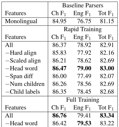
6.1 Feature Ablation

To verify that all our features were contributing to the model’s performance, we did an ablation study, removing one group of features at a time. Table 2 shows the F1 scores on the bilingual development data resulting from training with each group of fea-tures removed.7 Note that though head word fea-tures seemed to be detrimental in our rapid train-ing setup, earlier testtrain-ing had shown a positive effect, so we reran the comparison using our full training setup, where we again saw an improvement when including these features.

6

Available at http://nlp.cs.berkeley.edu.

7_{We do not have a test with the basic alignment features}

removed because they are necessary to computea0(t, t0).

Baseline Parsers Features Ch F1 Eng F1 Tot F1

Monolingual 84.95 76.75 81.15

Rapid Training Features Ch F1 Eng F1 Tot F1

All 86.37 78.92 82.91

−Hard align 85.83 77.92 82.16

−Scaled align 86.21 78.62 82.69

−Head word 86.47 79.00 83.00

−Span diff 86.00 77.49 82.07

−Num children 86.26 78.56 82.69

−Child labels 86.35 78.45 82.68 Full Training Features Ch F1 Eng F1 Tot F1

All 86.76 79.41 83.34

−Head word 86.42 79.53 83.22

Table 2: Feature ablation study. F1on dev set after

train-ing with individual feature groups removed. Performance with individual baseline parsers included for reference.

Ch F1 Eng F1 Tot F1 Tree Pairs 15 85.78 77.75 82.05 1,463,283 20 85.88 77.27 81.90 1,819,261 25 86.37 78.92 82.91 2,204,988 30 85.97 79.18 82.83 2,618,686 40 86.10 78.12 82.40 3,521,423 50 85.95 78.50 82.50 4,503,554

100 86.28 79.02 82.91 8,997,708

Table 3: Training set pruning study. F1 on dev set after

training with different values of theparameter for train-ing set pruntrain-ing.

6.2 Training Set Pruning

To find a good value of the parameter for train-ing set pruntrain-ing we tried several different values, us-ing our rapid trainus-ing setup and testus-ing on the dev set. The results are shown in Table 3. We selected 25 as it showed the best performance/speed trade-off, on average performing as well as if we had done no pruning at all, while requiring only a quarter the memory and CPU time.

6.3 Test Set Pruning

Cutoff Ch F1 Eng F1 Tot F1 Time (s)

50 86.34 79.26 83.04 174

100 86.61 79.31 83.22 307

200 86.67 79.39 83.28 509

500 86.76 79.41 83.34 1182

1000 86.80 79.39 83.35 2247

2000 86.78 79.35 83.33 4476

10,000 86.71 79.37 83.30 20,549

Table 4: Test set pruning study. F1on dev set obtained

using different cutoffs for test set pruning.

and testing on the dev set. The results are in Table 4. For F1 evaluation, which is on a very small set of sentences, we selected 500 as the value with the best speed/performance tradeoff. However, when rerank-ing our entire MT corpus, we used a value of 200, sacrificing a tiny bit of performance for an extra fac-tor of 2 in speed.8

6.4 Sensitivity tok

Since our bitext parser currently operates as a reranker, the quality of the trees is limited by the quality of thek-best lists produced by the baseline parsers. To test this limitation, we evaluated perfor-mance on the dev set using baselinek-best lists of varying length. Training parameters were fixed (full training setup withk= 100) and test set pruning was disabled for these experiments. The results are in Ta-ble 5. The relatively modest gains with increasingk, even as the oracle scores continue to improve, indi-cate that performance is limited more by the model’s reliance on the baseline parsers than by search errors that result from the reranking approach.

6.5 Final Results

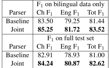
Our final evaluation was done using the full training setup. Here, we report F1scores on two sets of data. First, as before, we only include the sentence pairs from our bilingual corpus to fully demonstrate the gains made by joint parsing. We also report scores on the full test set to allow easier comparison with

8_{Using a rank cutoff of 200, the reranking step takes slightly}

longer than serially running both baseline parsers, and generat-ing k-best lists takes slightly longer than gettgenerat-ing 1-best parses, so in total, joint parsing takes about 2.3 times as long as mono-lingual parsing. With a rank cutoff of 500, total parsing time is scaled by a factor of around 3.8.

Joint Parsing Oracle k Ch F1 Eng F1 Ch F1 Eng F1

1 84.95 76.75 84.95 76.75

10 86.23 78.43 90.05 81.99

25 86.64 79.27 90.99 83.37

50 86.61 79.10 91.82 84.14

100 86.71 79.37 92.23 84.73

150 86.67 79.47 92.49 85.17

Table 5: Sensitivity tokstudy. Joint parsing and oracle

F1 obtained on dev set using different maximum values

ofkwhen generating baselinek-best lists.

F1 on bilingual data only Parser Ch F1 Eng F1 Tot F1 Baseline 83.50 79.25 81.44

Joint 85.25 81.72 83.52

F1on full test set Parser Ch F1 Eng F1 Tot F1 Baseline 82.91 78.93 81.00

Joint 84.24 80.87 82.62

Table 6: Final evaluation. Comparison of F1on test set

between baseline parsers and joint parser.

past work on Chinese parsing. For the latter evalu-ation, sentences that were not in the bilingual cor-pus were simply parsed with the baseline parsers. The results are in Table 6. Joint parsing improves F1by 2.5 points on out-of-domain English sentences and by 1.8 points on in-domain Chinese sentences; this represents the best published Chinese treebank parsing performance, even after sentences that lack a translation are taken into account.

7 Machine Translation

lan-Baseline Joint Moses

BLEU 18.7 21.1 18.8

Table 7: MT comparison on a syntactic system trained with trees output from either baseline monolingual parsers or our joint parser. To facilitate relative compari-son, the Moses (Koehn et al., 2007) number listed reflects the default Moses configuration, including its full distor-tion model, and standard training pipeline.

guage model for decoding. We tuned and evaluated BLEU (Papineni et al., 2001) on separate held-out sets of sentences of up to length 40 from the same corpus. The results are in Table 7, showing that joint parsing yields a BLEU increase of 2.4.9

8 Conclusions

By jointly parsing (and aligning) sentences in a translation pair, it is possible to exploit mutual con-straints that improve the quality of syntactic analy-ses over independent monolingual parsing. We pre-sented a joint log-linear model over source trees, target trees, and node-to-node alignments between them, which is used to select an optimal tree pair from a k-best list. On Chinese treebank data, this procedure improves F1 by 1.8 on Chinese sentences and by 2.5 on out-of-domain English sentences. Fur-thermore, by using this joint parsing technique to preprocess the input to a syntactic MT system, we obtain a 2.4 BLEU improvement.

Acknowledgements

We would like to thank the anonymous reviewers for helpful comments on an earlier draft of this paper and Adam Pauls and Jing Zheng for help in running our MT experiments.

References

Anthony Aue, Arul Menezes, Bob Moore, Chris Quirk, and Eric Ringger. 2004. Statistical machine trans-lation using labeled semantic dependency graphs. In TMI.

9

Note that all numbers are single-reference BLEU scores and are not comparable to multiple reference scores or scores on other corpora.

Ann Bies, Martha Palmer, Justin Mott, and Colin Warner. 2007. English chinese translation treebank v 1.0. Web download. LDC2007T02.

Daniel M. Bikel and David Chiang. 2000. Two statisti-cal parsing models applied to the chinese treebank. In Second Chinese Language Processing Workshop. Eugene Charniak and Mark Johnson. 2005.

Coarse-to-fine n-best parsing and maxent discriminative rerank-ing. InACL.

David Chiang. 2007. Hierarchical phrase-based

transla-tion. Computational Linguistics, 33(2):201–228.

Michael Collins. 2003. Head-driven statistical models

for natural language parsing. Computational

Linguis-tics, 29(4):589–637.

John DeNero and Dan Klein. 2007. Tailoring word

alignments to syntactic machine translation. InACL.

Yuan Ding and Martha Palmer. 2005. Machine trans-lation using probabilistic synchronous dependency

in-sertion grammars. InACL.

Michel Galley, Mark Hopkins, Kevin Knight, and Daniel

Marcu. 2004. What’s in a translation rule? In

HLT-NAACL.

Michel Galley, Jonathan Graehl, Kevin Knight, Daniel Marcu, Steve DeNeefe, Wei Wang, and Ignacio

Thayer. 2006. Scalable inference and training

of context-rich syntactic translation models. In

COLING-ACL.

Liang Huang, Kevin Knight, and Aravind Joshi. 2006. Statistical syntax-directed translation with extended

domain of locality. InHLT-NAACL.

Philipp Koehn, Hieu Hoang, Alexandra Birch, Chris Callison-Burch, Marcello Federico, Nicola Bertoldi, Brooke Cowan, Wade Shen, Christine Moran, Richard Zens, Chris Dyer, Ondrej Bojar, Alexandra Con-stantin, and Evan Herbst. 2007. Moses: Open source toolkit for statistical machine translation. InACL. Percy Liang, Ben Taskar, and Dan Klein. 2006.

Align-ment by agreeAlign-ment. InHLT-NAACL.

Yuval Marton and Philip Resnik. 2008. Soft syntactic constraints for hierarchical phrase-based translation. InACL.

Franz Josef Och, Daniel Gildea, Sanjeev Khudanpur, Anoop Sarkar, Kenji Yamada, Alex Fraser, Shankar Kumar, Libin Shen, David Smith, Katherine Eng, Viren Jain, Zhen Jin, and Dragomir Radev. 2003. Syn-tax for statistical machine translation. Technical re-port, CLSP, Johns Hopkins University.

Kishore Papineni, Salim Roukos, Todd Ward, and Wei-Jing Zhu. 2001. Bleu: a method for automatic eval-uation of machine translation. Research report, IBM. RC22176.

Slav Petrov and Dan Klein. 2007. Improved inference

Chris Quirk, Arul Menezes, and Colin Cherry. 2005. De-pendency treelet translation: Syntactically informed phrasal smt. InACL.

Libin Shen, Jinxi Xu, and Ralph Weishedel. 2008. A new string-to-dependency machine translation algo-rithm with a target dependency language model. In ACL.

David A. Smith and Noah A. Smith. 2004.

Bilin-gual parsing with factored estimation: using english

to parse korean. InEMNLP.

Leslie G. Valiant. 1979. The complexity of computing

the permanent. InTheoretical Computer Science 8.

Wen Wang, Andreas Stolcke, and Jing Zheng. 2007.

Reranking machine translation hypotheses with

struc-tured and web-based language models. InIEEE ASRU

Workshop.

Dekai Wu. 1997. Stochastic inversion transduction

grammars and bilingual parsing of parallel corpora. Computational Linguistics, 23(3):377–404.

Nianwen Xue, Fu-Dong Chiou, and Martha Palmer. 2002. Building a large-scale annotated chinese

cor-pus. InCOLING.

Kenji Yamada and Kevin Knight. 2001. A syntax-based statistical translation model. InACL.

Hao Zhang, Chris Quirk, Robert C. Moore, and

Daniel Gildea. 2008. Bayesian learning of

non-compositional phrases with synchronous parsing. In ACL.