NTUA SLP at IEST 2018: Ensemble of Neural Transfer Methods for Implicit Emotion Classification

Proceedings of the 9th Workshop on Computational Approaches to Subjectivity, Sentiment and Social Media Analysis, pages 57–64 57

NTUA-SLP at IEST 2018: Ensemble of Neural Transfer Methods for

Implicit Emotion Classification

Alexandra Chronopoulou1∗, Aikaterini Margatina1∗ Christos Baziotis1,2_{, Alexandros Potamianos}1,3

1_{School of ECE, National Technical University of Athens, Athens, Greece}

2_{Department of Informatics, Athens University of Economics and Business, Athens, Greece} 3_{Signal Analysis and Interpretation Laboratory (SAIL), USC, Los Angeles, USA}

[email protected], [email protected] [email protected], [email protected]

Abstract

In this paper we present our approach to tackle the Implicit Emotion Shared Task (IEST) or-ganized as part of WASSA 2018 at EMNLP 2018. Given a tweet, from which a certain word has been removed, we are asked to pre-dict the emotion of the missing word. In this work, we experiment with neural Transfer Learning (TL) methods. Our models are based on LSTM networks, augmented with a self-attention mechanism. We use the weights of various pretrained models, for initializing spe-cific layers of our networks. We leverage a big collection of unlabeled Twitter messages, for pretraining word2vec word embeddings and a set of diverse language models. Moreover, we utilize a sentiment analysis dataset for ptraining a model, which encodes emotion re-lated information. The submitted model con-sists of an ensemble of the aforementioned TL models. Our team ranked 3rdout of 30 partici-pants, achieving anF1score of 0.703.

1 Introduction

Social media, especially micro-blogging services like Twitter, have attracted lots of attention from the NLP community. The language used is con-stantly evolving by incorporating new syntactic and semantic constructs, such as emojis or hash-tags, abbreviations and slang, making natural lan-guage processing in this domain even more de-manding. Moreover, the analysis of such content leverages the high availability of datasets offered from Twitter, satisfying the need for large amounts of data for training.

∗

*These authors contributed equally to this work.

Emotion recognition is particularly interesting in social media, as it has useful applications in numerous tasks, such as public opinion detection about political tendencies (Pla and Hurtado,2014;

Tumasjan et al., 2010; Li and Xu, 2014), stock market monitoring (Si et al.,2013;Bollen et al.,

2011b), tracking product perception ( Chamlert-wat et al.,2012), even detection of suicide-related communication (Burnap et al.,2015).

In the past, emotion analysis, like most NLP tasks, was tackled by traditional methods that included hand-crafted features or features from sentiment lexicons (Nielsen, 2011; Mohammad and Turney, 2010, 2013; Go et al., 2009) which were fed to classifiers such as Naive Bayes and SVMs (Bollen et al., 2011a; Mohammad et al.,

2013; Kiritchenko et al., 2014). However, deep neural networks achieve increased performance compared to traditional methods, due to their abil-ity to learn more abstract features from large amounts of data, producing state-of-the-art re-sults in emotion recognition and sentiment anal-ysis (Deriu et al.,2016;Goel et al.,2017;Baziotis et al.,2017).

Twitter Dataset

Word2Vec Embeddings

Twitter Dataset

IEST Dataset

IEST Language Model Sentiment

Model Sentiment

Dataset

IEST Model Twitter

Dataset

Word2Vec Embeddings

Transfer Embeddings

Transfer Embeddings + Encoder Transfer

Embeddings

Language Model

IEST Dataset

Transfer Embeddings + Encoder

Finetuning P-Emb

P-Sent

P-LM

Figure 1: High-level overview of our TL approaches.

2 Overview

Our approach is composed of the following three steps: (1)pretraining, in which we train word2vec word embeddings Emb), a sentiment model Sent) and Twitter-specific language models (P-LM), (2) transfer learning, in which we transfer the weights of the aforementioned models to spe-cific layers of our IEST classifier and (3) ensem-bling, in which we combine the predictions of each TL model. Figure1depicts a high-level overview of our approach.

2.1 Data

Apart from the IEST dataset, we employ a Se-mEval dataset for sentiment classification and other manually-collected unlabeled corpora for our language models.

Unlabeled Twitter Corpora. We collected a dataset of 550 million archived English Twitter messages, from 2014 to 2017. This dataset is used for calculating word statistics for our text prepro-cessing pipeline and training ourword2vec word embeddings presented in Sec.4.1.

For training our language models, described in Sec. 4.3, we sampled three subsets of this cor-pus. The first consists of 2M tweets, all of which contain emotion words. To create the dataset, we selected tweets that included one of the six emo-tion classes of our task (anger, disgust, fear, joy, sadness andsurprise) or synonyms. We ensured that this dataset is balanced by concatenating ap-proximately 350K tweets from each category. The second chunk has 5M tweets, randomly selected from the initial 550M corpus. We aimed to create

a general sub-corpus, so as to focus on the struc-tural relationships of words, instead of their emo-tional content. The third chunk is composed of the two aforementioned corpora. We concatenated the 2M emotion dataset with 2M generic tweets, creating a final 4M dataset. We denote the three corpora asEmoCorpus(2M),EmoCorpus+ (4M) andGenCorpus(5M).

Sentiment Analysis Dataset. We use the dataset of SemEval17 Task4A (Sent17) (Rosenthal et al.,

2017) for training our sentiment classifier as de-scribed in Sec.4.2. The dataset consists of Twitter messages annotated with their sentiment polarity (positive, negative, neutral). The training set con-tains 56K tweets and the validation set 6K tweets.

2.2 Preprocessing

To preprocess the tweets, we useEkphrasis( Bazi-otis et al., 2017), a tool geared towards text from social networks, such as Twitter and Facebook.

Ekphrasis performs Twitter-specific tokenization, spell correction, word normalization, segmenta-tion (for splitting hashtags) and annotasegmenta-tion.

2.3 Word Embeddings

Word embeddings are dense vector representa-tions of words which capture semantic and syn-tactic information. For this reason, we employ the

word2vec(Mikolov et al.,2013) algorithm to train our word vectors, as described in Sec.4.1.

2.4 Transfer Learning

a related task by reducing the required training data (Torrey and Shavlik,2010;Pan et al.,2010). In computer vision, transfer learning is employed in order to overcome the deficit of training samples for some categories by adapting classifiers trained for other categories (Oquab et al.,2014). With the power of deep supervised learning, learned knowl-edge can even be transferred to a totally different task (i.e.ImageNet(Krizhevsky et al.,2012)).

Following this logic, TL methods have also been applied to NLP. Pretrained word vec-tors (Mikolov et al.,2013;Pennington et al.,2014) have become standard components of most ar-chitectures. Recently, approaches that leverage pretrained language models have emerged, which learn the compositionality of language, capture long-term dependencies and context-dependent features. For instance, ELMo contextual word representations (Peters et al.,2018) and ULMFiT (Howard and Ruder,2018) achieve state-of-the-art results on a wide variety of NLP tasks. Our work is mainly inspired by ULMFiT, which we extend to the Twitter domain.

2.5 Ensembling

We combine the predictions of our 3 TL schemes with the intent of increasing the generalization ability of the final classifier. To this end, we employ a pretrained word embeddings approach, as well as a pretrained sentiment model and a pretrained LM. We use two ensemble schemes, namely unweighted average and majority voting.

Unweighted Average (UA). In this approach, the final prediction is estimated from the unweighted average of the posterior probabilities for all differ-ent models. Formally, the final predictionpfor a training instance is estimated by:

p= arg max

c

1 C

M X

i=1

~

pi, pi ∈IRC (1)

whereCis the number of classes,Mis the number of different models, c ∈ {1, ..., C} denotes one class andp~iis the probability vector calculated by

modeli∈ {1, ..., M}using softmax function.

Majority Voting (MV). Majority voting approach counts the votes of all different models and chooses the class with most votes. Compared to UA, MV is affected less by single-network deci-sions. However, this schema does not consider any information derived from the minority mod-els. Formally, for a task with C classes and M

different models, the prediction for a specific in-stance is estimated as follows:

vc= M X

i=1

Fi(c)

p= arg max

c∈{1,...,C} vc

(2)

wherevcdenotes the votes for classcfrom all

dif-ferent models,Fiis the decision of theithmodel,

which is either 1 or 0 with respect to whether the model has classified the instance in classcor not andpis the final prediction.

3 Network Architecture

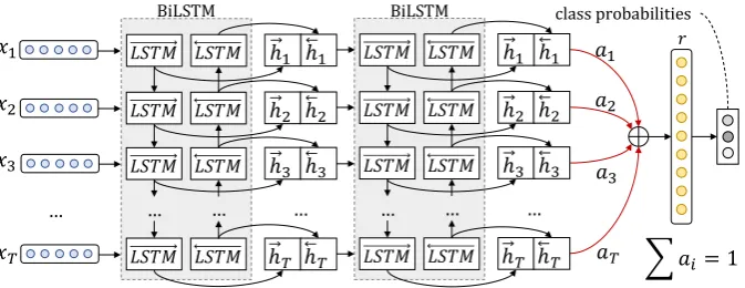
All of our TL schemes share the same architecture: A 2-layer LSTM with a self-attention mechanism. It is shown in Figure2.

Embedding Layer. The input to the network is a Twitter message, treated as a sequence of words. We use an embedding layer to project the words

w1, w2, ..., wN to a low-dimensional vector space

RW, whereW is the size of the embedding layer andN the number of words in a tweet.

LSTM Layer. An LSTM takes as input a se-quence of word embeddings and produces word annotationsh1, h2, ..., hN, wherehi is the hidden

state at time-stepi, summarizing all the informa-tion of the sentence up towi. We use bidirectional

LSTM to get word annotations that summarize the information from both directions. A bi-LSTM consists of a forward −→f that parses the sentence fromw1 towN and a backward

←−

f that parses it from wN to w1. We obtain the final annotation

for each wordhi, by concatenating the annotations

from both directions,hi =

− → hi k

←−

hi, hi ∈ R2L,

wherek denotes the concatenation operation and

L the size of each LSTM. When the network is initialized with pretrained LMs, we employ unidi-rectional instead of bi-LSTMs.

Attention Layer. To amplify the contribution of the most informative words, we augment our LSTM with an attention mechanism, which as-signs a weightaito each word annotationhi. We

compute the fixed representationrof the whole in-put message, as the weighted sum of all the word annotations.

ei =tanh(Whhi+bh), ei ∈[−1,1] (3)

ai =

exp(ei) PT

t=1exp(et)

,

T X

i=1

𝑥1 𝐿𝑆𝑇𝑀 𝐿𝑆𝑇𝑀 BiLSTM

𝑎1

𝑎𝑇 ෍ 𝑎𝑖= 1 ℎ1 ℎ1

𝑥2 𝐿𝑆𝑇𝑀 𝐿𝑆𝑇𝑀 ℎ2 ℎ2

𝑥3 𝐿𝑆𝑇𝑀 𝐿𝑆𝑇𝑀 ℎ₃ ℎ₃

𝑥𝑇 𝐿𝑆𝑇𝑀 𝐿𝑆𝑇𝑀 ℎ𝑇 ℎ𝑇

… …

𝐿𝑆𝑇𝑀 𝐿𝑆𝑇𝑀 BiLSTM

ℎ₁ ℎ₁

𝐿𝑆𝑇𝑀 𝐿𝑆𝑇𝑀 ℎ2 ℎ2

𝐿𝑆𝑇𝑀 𝐿𝑆𝑇𝑀 ℎ3 ℎ3

𝐿𝑆𝑇𝑀 𝐿𝑆𝑇𝑀 ℎ𝑇 ℎ𝑇

… …

𝑎2

𝑎3

… … …

classprobabilities 𝑟

Figure 2: The proposed model, composed of a 2-layer bi-LSTM with a deep self-attention mechanism. When the model is initialized with pretrained LMs, we use unidirectional LSTM instead of bidirectional.

r=

T X

i=1

aihi, r∈R2L (5)

whereWhandbhare the attention layer’s weights.

Output Layer. We use the representation r as feature vector for classification and we feed it to a fully-connected softmax layer with L neurons, which outputs a probability distribution over all classespcas described in Eq.6:

pc=

eW r+b

P

i∈[1,L](eWir+bi)

(6)

whereW andbare the layer’s weights and biases.

4 Transfer Learning Approaches

4.1 Pretrained Word Embeddings (P-Emb)

In the first approach, we train word2vec word embeddings with which we initialize the embed-ding layer of our network. The weights of the embedding layer remain frozen during training. The word2vec word embeddings are trained on the 550M Twitter corpus (Sec. 2.1), with nega-tive sampling of 5 and minimum word count of 20, using Gensim’s (Reh˚uˇrek and Sojkaˇ ,2010) im-plementation. The resulting vocabulary contains

800,000words.

4.2 Pretrained Sentiment Model (P-Sent)

In the second approach, we first train a sentiment analysis model on the Sent17 dataset, using the ar-chitecture described in Sec. 3. The embedding layer of the network is initialized with our pre-trained word embeddings. Then, we fine-tune the network on the IEST task, by replacing its last layer with a task-specific layer.

4.3 Pretrained Language Model (P-LM)

The third approach consists of the following steps: (1) we first train a language model on a generic Twitter corpus, (2) we fine-tune the LM on the task at hand and finally, (3) we transfer the embedding and RNN layers of the LM, we add attention and output layers and fine-tune the model on the target task.

LM Pretraining. We collect three Twitter datasets as described in Sec. 2.1and for each one we train an LM. In each dataset we use the 50,000 most frequent words as our vocabulary. Since the literature concerning LM transfer learning is limited, especially in the Twitter domain, we aim to explore the desired characteristics of the pre-trained LM. To this end, our contribution in this research area lies in experimenting with a task-relevant corpus (EmoCorpus), a generic one (Gen-Corpus) and a mixture of both (EmoCorpus+).

LM Fine-tuning. This step is crucial since, albeit the diversity of the general-domain data used for pretraining, the data of the target task will likely have a different distribution.

We thus fine-tune the three pretrained LMs on the IEST dataset, employing two approaches. The first is simple fine-tuning, according to which all layers of the model are trained simultane-ously. The second one is a simplified yet sim-ilar approach to gradual unfreezing, proposed in (Howard and Ruder, 2018), which we denote asSimplified Gradual Unfreezing(SGU). Accord-ing to this method, after we have transfered the pretrained embedding and LSTM weights, we let only the output layer fine-tune for n−1 epochs. At the nth _{epoch, we unfreeze both LSTM}

embed-ding layer and let the network train until conver-gence. In other words, we experiment with pairs of numbers of epochs, {n, k}, wherendenotes the epoch when we unfreeze the LSTM layers andk

the epoch when we unfreeze the embedding layer. Naive fine-tuning poses the risk of catastrophic forgetting, or else abruptly losing the knowledge of a previously learnt task, as information rele-vant to the current task is incorporated. Therefore, to prevent this from happening, we unfreeze the model starting from the last layer, which is task-specific, and after some epochs we progressively unfreeze the next, more general layers, until all layers are unfrozen.

LM Transfer. This is the final step of our TL ap-proach. We now have several LMs from the sec-ond step of the procedure. We transfer their em-bedding and RNN weights to a final target classi-fier. We again experiment with both simple and more sophisticated fine-tuning techniques, to find out which one is more helpful to this task.

Furthermore, we introduce the concatenation method which was inspired by the correlation of language modeling and the task at hand. We use pretrained LMs to leverage the fact that the task is basically a cloze test. In an LM, the probability of occurrence of each word, is conditioned on the preceding context,P(wt|w1, . . . , wt−1). In

RNN-based LMs, this probability is encoded in the hid-den state of the RNN,P(wt|ht−1). To this end, we

concatenate the hidden state of the LSTM, right before the missing word,himplicit, to the output of

the self-attention mechanism,r:

r0 =r khimplicit, hi ∈R2L (7)

whereLis the size of each LSTM, and then feed it to the output linear layer. This way, we pre-serve the information which implicitly encodes the probability of the missing word.

5 Experiments and Results

5.1 Experimental Setup

Training. We use Adam algorithm (Kingma and Ba, 2014) to optimize our networks, with mini-batches of size 64 and clip the norm of the gra-dients (Pascanu et al., 2013) at 0.5, as an extra safety measure against exploding gradients. We also used PyTorch (Paszke et al.,2017) and Scikit-learn (Pedregosa et al.,2011).

Hyperparameters. For all our models, we em-ploy the same 2-layer attention-based LSTM

ar-chitecture (Sec. 3). All the hyperparameters used are shown in Table1.

Layer P-Emb P-Sent P-LM

Embedding 300 300 400

Embedding noise 0.1 0.1 0.1 Embedding dropout 0.2 0.2 0.2 LSTM size 400 400 600/800 LSTM dropout 0.4 0.4 0.4

Table 1: Hyper-parameters of our models.

5.2 Official Results

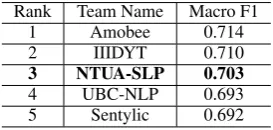
Our team ranked 3rdout of 30 participants, achiev-ing0.703F1-score on the official test set. Table2

shows the official ranking of the top scoring teams.

Rank Team Name Macro F1 1 Amobee 0.714 2 IIIDYT 0.710

3 NTUA-SLP 0.703

4 UBC-NLP 0.693 5 Sentylic 0.692

Table 2: Results of the WASSA IEST competition.

5.3 Experiments

Baselines. In Table 5 we compare the proposed TL approaches against two strong baselines: (1) a Bag-of-Words (BoW) model with TF-IDF weight-ing and (2) a Bag-of-Embeddweight-ings (BoE) model, where we retrieve the word2vec representations of the words in a tweet and compute the tweet representation as the centroid of the constituent

word2vec representations. Both BoW and BoE

features are then fed to a linear SVM classifier, with tunedC= 0.6. All of our reported F1-scores are calculated on the evaluation (dev) set, due to time constraints.

P-EmbandP-Sentmodels (4.1,4.2). We evaluate theP-EmbandP-Sentmodels, using both bidirec-tional and unidirecbidirec-tional LSTMs. The F1 score of our best models is shown in Table5. As expected, bi-LSTM models achieve higher performance.

LM Fine-tuning LM Transfer

Simple FT SGU Concat. F1

Simple FT

3 0.672

3 3 0.667

3 0.676

3 3 0.673

SGU

3 0.673

3 3 0.667

3 0.678

3 3 0.682

Table 3: Results of the P-LM, trained on the Emo-Corpus. The first column refers to the way we fine-tune each LM on the IEST dataset and the second to the way we finally fine-tune the classifier on the same dataset.

Dataset F1 EmoCorpus 0.682 EmoCorpus+ 0.680 GenCorpus 0.675

Table 4: Comparison of the P-LM models, all fine-tuned withSGUandConcat.methods.

GenCorpus corpora, (2)LM fine-tuning: we fine-tune the LMs on the IEST dataset, with 2 different ways. The first one is simple fine-tuning, while the second one is our simplified gradual unfreezing (SGU) technique. (3)LM transfer: We now have 6 LMs, fine-tuned on the IEST dataset. We trans-fer their weights to our final emotion classifier, we add attention to the LSTM layers and we experi-ment again with our 2 ways of fine-tuning and the

concatenation methodproposed in Sec.4.3. In Table3we present all possible combinations of transferring the P-LM to the IEST task. We observe that SGU consistently outperforms Sim-ple Fine-Tuning (SimSim-ple FT). Due to the difficulty in running experiments for all possible combina-tions, we compare our best approach, namelySGU

+ Concat., with P-LMs trained on our three un-labeled Twitter corpora, as depicted in Table 4. Even though EmoCorpus contains less training ex-amples,P-LMs trained on it learn to encode more useful information for the task at hand.

5.4 Ensembling

Our submitted model is an ensemble of the mod-els with the best performance. More specifically, we leverage the following models: (1) TL of pre-trained word embeddings, (2) TL of prepre-trained sentiment classifier, (3) TL of 3 different LMs, trained on 2M, 4M and 5M respectively. We use Unweighted Average (UA) ensembling of our best

Model F1

Bag of Words (BoW) 0.601 Bag of Embeddings (BoE) 0.605

P-Emb 0.668

P-Sent 0.671

P-LM 0.675

P-Emb + bidir. 0.684 P-Sent + bidir. 0.674

P-LM + SGU 0.679

P-LM + SGU + Concat. 0.682 Ensembling (UA) P-Emb + P-Sent 0.684 Ensembling (UA) P-Sent + P-LM 0.695 Ensembling (UA) P-Emb + P-LM 0.701 Ensembling (MV) All 0.700 Ensembling (UA) All 0.702

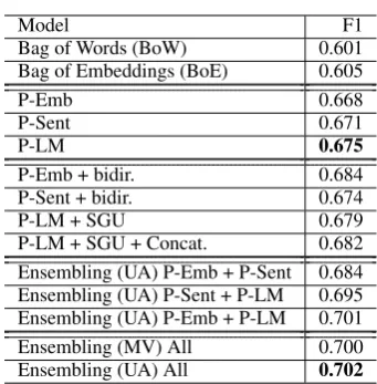
Table 5: Results of our experiments when tested on the evaluation (dev) set. BoW and BoE are our baselines, whileP-Emb,P-SentandP-LMour proposed TL approaches. SGU stands for Sim-plified Gradual Unfreezing, bidir. for bi-LSTM,

Concat.for the concatenation method,UAfor Un-weighted Average andMVfor Majority Voting en-sembling.

models from all aforementioned approaches. Our final results on the evaluation data are shown in Table5.

5.5 Discussion

As shown in Table 5, we observe that all of our proposed models achieve individually better per-formance than our baselines by a large margin. Moreover, we notice that, when the three mod-els are trained with unidirectional LSTM and the same number of parameters, the P-LM outper-forms both theP-Emband theP-Sentmodels. As expected, the upgrade to bi-LSTM improves the results ofP-EmbandP-Sent. We hypothesize that

P-LMwith bidirectional pretrained language mod-els would have outperformed both of them. Fur-thermore, we conclude that both SGU for fine-tuning and the concatenation method enhance the performance of theP-LMapproach. As far as the ensembling is concerned, both approaches, MV

6 Conclusion

In this paper we describe our deep-learning meth-ods for missing emotion words classification, in the Twitter domain. We achieved very competitive results in the IEST competition, ranking 3rd/30 teams. The proposed approach is based on an ensemble of Transfer Learning techniques. We demonstrate that the use of refined, high-level fea-tures of text, as the ones encoded in language mod-els, yields a higher performance. In the future, we aim to experiment with subword-level mod-els, as they have shown to consistently face the OOV words problem (Sennrich et al.,2015; Bo-janowski et al., 2016), which is more evident in Twitter. Moreover, we would like to explore other transfer learning approaches.

Finally, we share the source code of our mod-els1, in order to make our results reproducible and facilitate further experimentation in the field.

References

Christos Baziotis, Nikos Pelekis, and Christos Doulk-eridis. 2017. Datastories at semeval-2017 task 4: Deep lstm with attention for message-level and topic-based sentiment analysis. In Proceedings of the 11th International Workshop on Semantic Eval-uation (SemEval-2017), pages 747–754.

Piotr Bojanowski, Edouard Grave, Armand Joulin, and Tomas Mikolov. 2016. Enriching word vec-tors with subword information. arXiv preprint arXiv:1607.04606.

Johan Bollen, Huina Mao, and Alberto Pepe. 2011a. Modeling public mood and emotion: Twitter sen-timent and socio-economic phenomena. Icwsm, 11:450–453.

Johan Bollen, Huina Mao, and Xiaojun Zeng. 2011b. Twitter mood predicts the stock market. Journal of computational science, 2(1):1–8.

Pete Burnap, Walter Colombo, and Jonathan Scour-field. 2015. Machine classification and analysis of suicide-related communication on twitter. In Pro-ceedings of the 26th ACM conference on hypertext & social media, pages 75–84. ACM.

Wilas Chamlertwat, Pattarasinee Bhattarakosol, Tip-pakorn Rungkasiri, and Choochart Haruechaiyasak. 2012. Discovering consumer insight from twitter via sentiment analysis.J. UCS, 18(8):973–992.

Jan Deriu, Maurice Gonzenbach, Fatih Uzdilli, Au-relien Lucchi, Valeria De Luca, and Martin Jaggi.

1_{/github.com/alexandra-chron/}

wassa-2018

2016. Swisscheese at semeval-2016 task 4: Senti-ment classification using an ensemble of convolu-tional neural networks with distant supervision. In Proceedings of the 10th international workshop on semantic evaluation, EPFL-CONF-229234, pages 1124–1128.

Alec Go, Richa Bhayani, and Lei Huang. 2009. Twit-ter sentiment classification using distant supervision. CS224N Project Report, Stanford, 1(12).

Pranav Goel, Devang Kulshreshtha, Prayas Jain, and Kaushal Kumar Shukla. 2017. Prayas at emoint 2017: An ensemble of deep neural architectures for emotion intensity prediction in tweets. In Pro-ceedings of the 8th Workshop on Computational Ap-proaches to Subjectivity, Sentiment and Social Me-dia Analysis, pages 58–65.

Jeremy Howard and Sebastian Ruder. 2018. Fine-tuned language models for text classification.CoRR, abs/1801.06146.

Diederik Kingma and Jimmy Ba. 2014. Adam: A method for stochastic optimization. arXiv preprint arXiv:1412.6980.

Svetlana Kiritchenko, Xiaodan Zhu, and Saif M. Mo-hammad. 2014. Sentiment analysis of short in-formal texts. Journal of Artificial Intelligence Re-search, 50:723–762.

Roman Klinger, Orphée de Clercq, Saif M. Moham-mad, and Alexandra Balahur. 2018. Iest: Wassa-2018 implicit emotions shared task. InProceedings of the 9th Workshop on Computational Approaches to Subjectivity, Sentiment and Social Media Anal-ysis, Brussels, Belgium. Association for Computa-tional Linguistics.

Alex Krizhevsky, Ilya Sutskever, and Geoffrey E Hin-ton. 2012. Imagenet classification with deep con-volutional neural networks. In Advances in neural information processing systems, pages 1097–1105.

Weiyuan Li and Hua Xu. 2014. Text-based emotion classification using emotion cause extraction. Ex-pert Systems with Applications, 41(4):1742–1749.

Tomas Mikolov, Ilya Sutskever, Kai Chen, Greg S. Cor-rado, and Jeff Dean. 2013. Distributed representa-tions of words and phrases and their compositional-ity. InAdvances in Neural Information Processing Systems, pages 3111–3119.

Saif M. Mohammad, Svetlana Kiritchenko, and Xiao-dan Zhu. 2013. NRC-Canada: Building the state-of-the-art in sentiment analysis of tweets. arXiv preprint arXiv:1308.6242.

Saif M Mohammad and Peter D Turney. 2013. Crowd-sourcing a word–emotion association lexicon. Com-putational Intelligence, 29(3):436–465.

Finn Årup Nielsen. 2011. A new anew: Evaluation of a word list for sentiment analysis in microblogs. arXiv preprint arXiv:1103.2903.

Maxime Oquab, Leon Bottou, Ivan Laptev, and Josef Sivic. 2014. Learning and transferring mid-level im-age representations using convolutional neural net-works. In Proceedings of the IEEE conference on computer vision and pattern recognition, pages 1717–1724.

Sinno Jialin Pan, Qiang Yang, et al. 2010. A survey on transfer learning. IEEE Transactions on knowledge and data engineering, 22(10):1345–1359.

Razvan Pascanu, Tomas Mikolov, and Yoshua Bengio. 2013. On the difficulty of training recurrent neural networks. ICML (3), 28:1310–1318.

Adam Paszke, Sam Gross, Soumith Chintala, Gre-gory Chanan, Edward Yang, Zachary DeVito, Zem-ing Lin, Alban Desmaison, Luca Antiga, and Adam Lerer. 2017. Automatic differentiation in pytorch.

Fabian Pedregosa, Gaël Varoquaux, Alexandre Gram-fort, Vincent Michel, Bertrand Thirion, Olivier Grisel, Mathieu Blondel, Peter Prettenhofer, Ron Weiss, Vincent Dubourg, and others. 2011. Scikit-learn: Machine learning in Python. Journal of Ma-chine Learning Research, 12(Oct):2825–2830.

Jeffrey Pennington, Richard Socher, and Christo-pher D. Manning. 2014. Glove: Global Vectors for Word Representation. InEMNLP, volume 14, pages 1532–1543.

Matthew E Peters, Mark Neumann, Mohit Iyyer, Matt Gardner, Christopher Clark, Kenton Lee, and Luke Zettlemoyer. 2018. Deep contextualized word rep-resentations. arXiv preprint arXiv:1802.05365.

Ferran Pla and Lluís-F Hurtado. 2014. Political ten-dency identification in twitter using sentiment anal-ysis techniques. In Proceedings of COLING 2014, the 25th international conference on computational linguistics: Technical Papers, pages 183–192.

Radim ˇReh˚uˇrek and Petr Sojka. 2010. Software Framework for Topic Modelling with Large Corpora. In Proceedings of the LREC 2010 Workshop on New Challenges for NLP Frame-works, pages 45–50, Valletta, Malta. ELRA. http://is.muni.cz/publication/

884893/en.

Sara Rosenthal, Noura Farra, and Preslav Nakov. 2017. Semeval-2017 task 4: Sentiment analysis in twitter. In Proceedings of the 11th International Workshop on Semantic Evaluation (SemEval-2017), pages 502–518.

Rico Sennrich, Barry Haddow, and Alexandra Birch. 2015. Neural machine translation of rare words with subword units. arXiv preprint arXiv:1508.07909.

Jianfeng Si, Arjun Mukherjee, Bing Liu, Qing Li, Huayi Li, and Xiaotie Deng. 2013. Exploiting topic based twitter sentiment for stock prediction. In Pro-ceedings of the 51st Annual Meeting of the Associa-tion for ComputaAssocia-tional Linguistics (Volume 2: Short Papers), volume 2, pages 24–29.

Lisa Torrey and Jude Shavlik. 2010. Transfer learn-ing. InHandbook of Research on Machine Learning Applications and Trends: Algorithms, Methods, and Techniques, pages 242–264. IGI Global.