Unknown Input High Gain Observer for Parametric Fault Detection and Isolation of Dynamical Systems

(1)

Unknown Input High Gain Observer for

Parametric Fault Detection and Isolation of

Dynamical Systems

Sharifuddin Mondal*, Goutam Chakraborty and Kingshook Bhattacharyya

Abstract: An unknown input high gain observer based parametric fault detection and isolation scheme is presented. First, a reduced order unknown input high gain observer is derived. Then, using these observers, a fault detection and isolation technique is devised to detect and isolate the parametric fault of a system whose parameters are uncertain to some extent. The proposed FDI algorithm consists of two steps. In the first step, the detection of fault and the isolation of faulty region are achieved and in the next step, the faulty parameter is isolated from the faulty region. Effectiveness of the observer as well as the FDI technique is shown with the help of a numerical example.

Keywords: Unknown input high gain observer; parametric fault; fault detection and isolation; parameter estimation.

I. INTRODUCTION

With the rising demands of high reliability and safety of advanced processes like avionics, nuclear power stations, automobiles etc have led to increasing requirements of developing new methods for supervision and monitoring as a part of overall process control scheme. Different fault detection and isolation (FDI) schemes have been developed for avoiding failure of the plants. Model based fault detection techniques (like Kalman filter or observer based) have received increasing attention following the pioneering work of Beard [1].

The FDI concept using observers or Kalman filters is based on the assumption that the mathematical model of the system is perfectly known. In reality, however this assumption does not hold, because the

Manuscript received December 29, 2008.

S. Mondal is with the Department of Mechanical Engineering, Pohang University of Science and Technology, Pohang, 790 784, South Korea, Tel. No. +82-54 2795908, Fax. +82-54-2798459, e-mail: [email protected]

G. Chakraborty and K. Bhattacharyya are with the Department of Mechanical Engineering, Indian Institute of Technology, Kharagpur, Pin- 721302, India, e-mails: [email protected], [email protected].

* Corresponding author

parameters of a process are in general uncertain or time varying. Again the characteristics of disturbances or noise are not completely known; hence they cannot be perfectly modeled. There is always a mismatch between the actual process model and its mathematical model (even if there is no fault in the process), which sometimes produces false alarms corrupting the performance of the FDI process. To avoid false alarms, the FDI method should be made robust i.e., insensitive to modeling uncertainties. But the algorithm should not be too robust to ignore the fault i.e., a significantly large variation of the parameter values.

Over the years, various kinds of robust fault detection and isolation techniques have been developed to diagnose different types of faults like sensors, actuators or components [2, 5, 7, 8, 12, 13]. Frank [6], in a survey paper, described different types of observer based robust fault diagnosis techniques. Patton and Chen [11] discussed various robustness issues related observer based fault diagnosis techniques. Linear matrix inequality (LMI) based robust fault detection techniques for uncertain systems have been developed in [14]. The identification based FDI techniques have been used by many researchers [9] for different types of fault diagnosis. Daley and Wang [3] used a high gain observer, which was developed by Petersen and Hollot [10], as a tool for sensor fault detection.

(2)

work, a part of the system parameters (i.e., the parameters of the faulty subsystem) is estimated and only when a fault occurs in the system. In this respect the complexity of fault isolation is drastically reduced in comparison with standard parameter identification technique [9]where all the parameters of a system are estimated at every instant and compared with actual values. A numerical example is presented to show the effectiveness of the observer as well as the FDI technique.

The basic methodology of designing the unknown input high gain observer for an uncertain system is discussed in section II. The fault detection and isolation algorithm is explained in section III. A numerical example is presented in section IV. The concluding remarks are included in section V.

II. UNKNOWN INPUT HIGH GAIN OBSERVER

In this section, an unknown input high gain observer is developed. The sufficient conditions for existence of such observers are provided.

Consider a linear time-invariant uncertain system with unknown inputs

( )t =( + ∆ ) ( )t +( + ∆ ) ( )t + ( )

x A A x B B u Ed t

t

(1)

( )t = ( )

y Cx . (2)

where - the state vector, - the

measurable input vector,

( )t ∈ n

x R ( ) m

t ∈

u R

( ) p

t ∈

y R - the output vector

and - the unknown input vector. The

matrices and

( )t ∈ q

d R

, ,

A B C E of suitable dimensions are known. The matrices ∆ and ∆ are the uncertainties of the system and input matrices. It is assumed that

is always asymptotically stable for all

A B

(A+ ∆A) ∆A.

It is assumed that the system satisfies the rank condition: rank(CE)=rank(E).

t

Now, using a state transformation matrix T, the states are redefined as z( )t =Tx( ) such that

( )

2

n r− ×q

⎡ = ⎢ ⎣ ⎦ TE E φ ⎤

⎥ where E2 is dimensional matrix with

r q

×

2

( ) ( )

rank E =rank E and

φ

is a null matrix. The system and output equations can be recast as follows

( )

1 11 12 1 1

2 21 22 2 2 2

1 1

11 12

2 2

21 22

n r− ×q

⎡ ⎤ ⎡ ⎤ ⎡ ⎤ ⎧ ⎫₌ ⎧ ⎫₊ ₊ ⎨ ⎬ ⎢ ⎥⎨ ⎬ ⎢ ⎥ ⎢ ⎥ ⎩ ⎭ ⎣ ⎦⎩ ⎭ ⎣ ⎦ ⎣ ⎦ ⎡∆ ∆ ⎤⎧ ⎫ ⎡∆ ⎤ +_⎢ _⎥_{⎨ ⎬}+_⎢ _⎥ ∆ ∆ ∆ _{⎩ ⎭ ⎣} _⎦ ⎣ ⎦

z A A z B

u d

z A A z B E

z B A A u z B A A φ (3) 1 1 2 2 ( )t =⎡_⎣ ⎤⎧ ⎫_{⎨ ⎬}

⎦ ⎩ ⎭z

y C C

z

. (4)

Now it is assumed that the measurement signals are such that the following rank condition is satisfied:

. This is a necessary condition for

designing this observer as the extra measurement signals are used to design the reduced order observer after decoupling the unknown inputs.

( ) ( )

rank C >rank

This condition allows the rearrangement of the output equation in the following form with the help of

a transformation 1 2 = ⎡ ⎤ ⎢ ⎥ ⎣ ⎦ y Vy y

, where V is a nonsingular

matrix, as

1 11

2 21 22 2

=⎡ ⎤ 1

⎧ ⎫ ⎧ ⎫ ⎨ ⎬ ⎢ ⎥ ⎩ ⎭ ⎣ ⎦⎩ ⎭⎨ ⎬

y C z

y C C z

φ _{. (5)}

Now the equations (3) and (5) can be written in expanded form as follows

1= 11 1+ 12 2+ 1 +∆ 11 1+∆ 12 2+∆ 1

z A z A z B u A z A z B u (6)

2= 21 1+ 22 2+ 2 + 2 +∆ 21 1+ 22 2+∆ 2

z A z A z B u E d A z A z B u (7)

1= 11

y C z1 (8)

2= 21 1+ 22

y C z C z2. (9)

Eliminating

z

₂ from the equation (6) by using the equation (9), one can get

1

1 11 1 12 22 2 21 1 1 11 1

12 2 1

( ) − _∆ ∆ ∆ = + − + + + +

z A z A C y C z B u A z

A z B u

. (10)

It can be seen that 1 22

−

C should be nonsingular, which will be always so as rank(CE)=rank( )E .

Now, the equation (10) can be written in a simplified form as

1= s 1+ s + u

_u

z A z B u E d , (11)

where ₁₁ ₁₂ ₂₂ 1 ₂₁

s

−

= −

A A A C C , 1

1 12 22

s

−

⎡ ⎤

= ⎣ ⎦

B B A C ,

2 =⎧ ⎫_{⎨ ⎬} ⎩ ⎭ u u y

and E d_u _u =∆A z_{11 1}+∆A z_{12 2}+∆B u₁ with E_u- known matrix and d_u- unknown signal.

For designing an observer, the system should satisfy the observability conditions: rank O( ( ,A C))=n. Now one can design an observer for the system (11) and (8) as

1 1 1 ˆ

ˆ = _sˆ + _s + ( −

1)

z A z B u K y y (12)

1 11 ˆ ₌ _ˆ

y C z₁. (13) The gain matrix is found out by solving the

following algebraic Riccati equation [3,10] K

2

11 11 2 0

T T

T u u T u u

s s

q

+ + + − + =

σ σ

E E PE E P

A P PA Q PC C P

(14) with ₌ ₁₁T

K PC , (15) where is a pre-chosen positive definite matrix and the constants q &

Q

σ are specified numbers. It was shown in [10] that for any , there exists q such that gain obtained from the above equations will lead to

0 σ >

11(jw − s+ 11) u&< σ

&C I A KC E for ∀ ∈w R1 where is the frequency. This condition implies that the

w

(3)

effect of unknown signal becomes very small in error dynamics for an appropriate value of

u

d

σ. The states

z

ˆ

₂ are estimated from equation (9) as

1

2 22 2 21 1

ˆ = −( − ˆ )

z C y C z . (16)

Now using zˆ=

{

zˆ₁ zˆ₂

}

T the estimated state vector

is found out as .

ˆ

x

1 ˆ= − ˆ

x T z

III. FAULT DETECTION AND ISOLATION ALGORITHM

In this section, a parametric fault detection and isolation technique for an uncertain system is described. It consists of two steps. In the first step, a set of residuals is generated with the help of a bank of high gain observers to detect the fault and isolate the faulty zone. In the second step, faulty parameter is isolated from the faulty zone.

Consider a linear time invariant system as

( )t =( + ∆ ) ( ) (t + + ∆ ) ( )

x A A x B B u t

t

(17) where the significance of the matrices and vectors are same as described in the previous section.

Suppose a parametric fault occurs in the plant. The detection and isolation of the fault are carried out in two steps as follows.

Step-1: Detection and partial isolation of fault The faulty system is written as

( )t =( + ∆ f + ∆ ) ( )t +( + ∆ f + ∆ ) ( )

x A A A x B B B u , (18) where ∆A_f and ∆Bf are the faulty parts of the

matrices A and B respectively. The state equation (18) can now be rearranged as

( )t =( + ∆ ) ( )t +( + ∆ ) ( )t + ( )

x A A x B B u Ed t , (19)

where E is a known matrix and is the

unknown input satisfying the relation

( )t ∈ q

d R

( )t = ∆ f ( )t + ∆ f ( )t

Ed A x B u . (20)

Now the system is divided into N number of subsystems with each characterized by a few parameters. The choice of subsystems is arbitrary. In a physical system, the subsystems are chosen based on the physical proximity of different parameters. Assume that the fault has occurred in the i-th subsystem. The system equations considering the fault in the i-th subsystem is written as

( )i( )t =( + ∆ ) ( )i ( )t +( + ∆ ) ( )t + ( ) ( )( )

x A A x B B u E d_i _i t

t

ˆ t

(21)

where the subscript (i) indicates that the fault has occurred only in the i-th subsystem.

The output equation for this system is written as

( )i( )t = ( )i ( )i ( )

y C x , (22) The equations (21) and (22) are similar to equations (1) and (2). Now, following the procedure discussed in

the previous section, an unknown input high gain observer is designed to estimate the states xˆ ( )_{( )}_i t .

Once the states are estimated, the residuals

are calculated as ( ) ˆ ( )_i t

x

( )i ( )t = ( )i( )t −ˆ( )i ( )t = ( )i( )t − ( )i ( )i ( )

r y y y C x . (23) Now, an unknown input observer, if properly

designed, can estimate the states irrespective of unknown inputs. So the residual , calculated

from the equation (23), converges within bounded value (i.e., threshold value) if the fault occurs in the i -th subsystem or -there is no fault in -the system as -the effect of possible faults in i-th is considered as unknown inputs. In this way, one can detect a fault and isolate the faulty subsystem using number of UIHGOs. However (

( )i ( )t

r

N 1

N− ) such observers will be sufficient to isolate a faulty subsystem when because once (

2 N> 1

N− ) subsystems are found fault free, the remaining subsystem is automatically identified as the faulty one. A decision table is drawn to isolate the faulty subsystem from observation of (N−1)

residuals.

Step-2: Total isolation of fault

In this step, the faulty parameter in the faulty subsystem is isolated. The effect of the faulty subsystem is now simulated as an unknown input signal, say . The relationship between , the parameters of the faulty subsystem, say , and the states are known and can be written as

( )

u

F t F t_u( )

s

( )t

x

,

( ) ( ) u

F t = f s x , (24) where the function ‘f ’ is linear for a linear system.

The system equation for this case becomes

( )t =( + ∆ ) ( )t +( + ∆ ) ( )t + ( )t

x A A x B B u Ed , (25) where d( )t =F t_u( ). With a measurement matrix , an

observer is then designed to estimate the states. Knowing the states, the unknown input signal is then estimated from the state equations neglecting the uncertainties using the nominal values of the parameters of the other non-faulty subsystems.

C

The estimated signal F tˆ ( )_u is now used to estimate the parameters 's from the relation (24) as

s

ˆ_{( )} _{( , ( ))}_ˆ u

F t = f s xt . (26)

Different parameter estimation techniques can be used to estimate from equation (26). However, a very simple logical estimation approach is applied in the present work in order to isolate the faulty element.

s

Let us consider the k-th parameter as the faulty

one. From the above relation, can be estimated using nominal values of rest of the parameters. Mathematically,

k

s

k

(4)

1 2 1 1 ˆ ˆ ˆk ( , ,..., k , k ,..., ( ), u( ))

s =g s s s− s+ x t F t (27) C1=3500 Ns / m where g is a functional.

In steady state, the estimated values vary very less if the assumption is correct. The moving averages technique is used to smoothen the fluctuation of the estimated values. If the assumption is wrong, the estimated values will vary significantly large. Now, as the single fault case is being considered, there will be only one case when the estimated parameter will vary less. The particular parameter for which it happens is the faulty one. In this way, the faulty parameter is isolated. With this the isolation process is completed. In this way, any parametric fault can be detected and isolated following the above two steps.

IV. NUMERICAL EXAMPLE

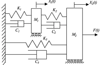
Consider a mechanical system as shown in figure 1. The state space model of the system can be written as follows:

x( )t =(A+ ∆A x) ( )t +(B+ ∆B u t) ( ), where

1 2 2 1 2 2

1 1 1 1

2 3 2 3

2 2

3 3 3

0 0 1 0

0 0 0 1

( ) ( )

( ) (

K K K C C C

M M M M

K K C C

K C

M M M M

⎡

3

)

⎢

⎢ ⎥

⎢₋ + ₋ + ⎥

⎢ ⎢

⎢ ₋ + ₋ +

⎢ ⎣

A =

⎤ ⎥

⎥ ⎥ ⎥ ⎥ ⎦ ,

,

[

0 0 0 (1/ 3)

]

T M

=

B

{

1 2 1 2

}

T

X X X X

=

x ,

, where

( )t =F t( )

u X_i and X_i are the displacement

and velocity of the mass element M_i respectively,

j

K - the stiffness element and C_j- the damping coefficient (i=1,2 and j=1, 2, 3). The matrices ∆A and

are uncertainties.

[image:4.612.91.285.503.629.2]

∆B

Figure 1: Mechanical system having two masses and three sets of spring-damper

The numerical values of the parameters are

, , ,

, ,

1 870 kg

M = M₃=1550 kg K₁=280000 N / m 2 370000 N / m

K = K₃=340000 N / m

, C₂ =3000 Ns / m and

3 5675 Ns / m

C = .

A fault is introduced at in the spring of stiffness

50 sec

t=

2

K . The new value of K₂ is set to 185000 N/m. Now using FDI algorithm, discussed in section 3, the fault (hereK₂) is detected and isolated as follows.

Step-1: Detection and partial isolation of the fault First, the system is divided into three subsystems as follows: SS1:K₁, C₁ & M₁; SS2:K₂ & and

:

2

C

SS3 K₃, C₃ & M₃.

The uncertainties are as follows: ∆ =A M NΣ ₁ and 2

∆ =B M NΣ with M =In, N1=0.05×Au,

2=0.05× u

N B and Σ Σ= ₀sin(w t₁) where

0=0.25×I

Σ and w₁=0.05 rad/s. The matrices and

u

A

u

B are same as A and excepting the elements containing constant terms are replaced with zeros. The sinusoidal variation in system parameters is applied. The following input signal is applied in numerical simulation:

B

0 in( )

u s wt =

0 0 1

]

T

u =

E and

[

]

(3) 0 0 1

T u =

E . The tuning parameters

σ

and

are considered as

q

(1) 0.05

σ = , σ₍₃₎=0.05,

q

₍₁₎

=

15

and q₍₃₎=15. The value of Q is chosen as for both the observers.

1

5 n

=

Q I

Two high gain observers are then designed for the above systems and the gain matrices are calculated from the equations (14) and (15). The values of the observer gains for the above observers are

[

]

(1) 0.7253 4.7760 14.8934

T

=

K and

[

]

(3) 0.4368 2.9387 -13.1569

T

=

K respectively. The

residuals are plotted in figure 2 and figure 3.

(5)

uncertainties. Hence two small threshold values

{

5 2

}

(1) 1.5 10 1 10

T

ε ₌ _× − _× −0 _and

{

9 2

}

(3) 3 10 3 10

T

[image:5.612.101.287.146.391.2]

ε _{= ×} − _× −0 units are chosen. These are calculated when there is no fault in the system.

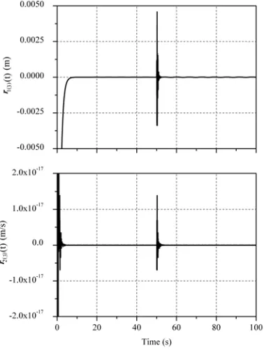
Figure 2: Components of the residual

r

₍₁₎

( )

t

Figure 3: Components of the residual

r

₍₃₎

( )

t

[image:5.612.312.548.151.228.2]

As both the residuals cross the threshold values, the existence of fault is confirmed. In order to isolate the faulty subsystem a decision table is constructed as shown in table 2.

Table 1: Decision table for isolation of faulty subsystem

Is r_(i)>

ε

_(i) (use ‘1’) or

(i)

≤

(i)

r

ε

(use ‘0’) ? Observation

(1)

r

₍₃₎

Decision

Case 1 1 Fault: SS2.

From table-1, it is seen that the fault is in subsystem 2. Now the next step (i.e., step-2) is carried out to isolate faulty parameter.

Step-2: Total isolation of the fault

Here the faulty subsystem (SS2) is replaced by an unknown force F tu( ) as

F t_u( )=K₂(X₂−X₁)+C X₂( ₂−X₁).

The system is remodeled as follows

( )t =( + ∆ ) ( )t +( + ∆ ) ( )t + ( )t

x A A x B B u Ed

where E=

[

0 0 1/M₁ −1/M3

]

T and ( )d t =F tu( ).

It can be noticed that the parameter uncertainties for this system are only in 3rd and 4th rows of A and B matrices for this problem, which indicate ∆A and ∆B have non-zero elements in 3rd and 4th rows only. For this advantage here the system equation can be rewritten combining the unknown inputs and uncertainties as

( )x t =Ax( )t +Bu( )t +E dc c( )t

whereE_c=

[

0 0 1 0; 0 0 0 1

]

Tand

3,1 4 3,1 / 1 4,1 4 4,1 / 3

T c= ∆⎣⎡ − + ∆ +Fu M ∆ − + ∆ −Fu M ⎤⎦

d A x B u A x B u .

This special situation may not occur in all system. A full order unknown input observer [4] is designed with output matrix C=

[

0 1 2 0; 0 0−1 1;1 0 0 0

]

T to estimate the states . Using the estimated states

and the nominal values of the parameters of subsystem-1, the unknown input

ˆ ( )t

x

ˆ ( )t

x

( ) u

F t is estimated

from the following relationship ˆ_{( )} ₁_ˆ₃ ₁_ˆ₁ ₁ ₃,

u

F t =M x +K x +Cxˆ

where is calculated taking the derivative of with respect to time.

3 ˆ

x xˆ3

Finally the faulty parameters are estimated using the following relation

ˆ_{( )} ₂₍_ˆ₂ _ˆ₁₎ ₂₍_ˆ₄ _ˆ₃₎ u

F t =K x −x +C x −x

First, the fault is assumed in and the stiffness

is estimated using the nominal value of =3000 2

K K₂

2

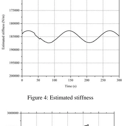
[image:5.612.98.287.435.686.2]

(6)

Ns/m. The moving averages are taken to smoothen the estimated values and the estimated values are plotted in figure 4. The plot shows that estimated values vary very less from it mean value. Now is assumed to be faulty and is estimated using the nominal value of

2

C

2

C

2

K =370000 N/m. The estimated values after taking

moving averages are plotted in figure 5. The plot shows that the estimated values of vary widely, which is because of wrong assumption. This confirms that fault is in

2

C

2

K and thereby the fault isolation

[image:6.612.85.297.242.460.2]

process is completed.

[image:6.612.86.288.423.587.2]

Figure 4: Estimated stiffness

Figure 5: Estimated damping coefficient

Thus it is seen that the FDI scheme works well for the occurrence of fault in subsystem 2. It can be shown easily that the method works with equal ease for any parameter fault in other subsystem.

V. CONCLUSIONS

An UIHGO based parameter FDI scheme is presented. First an UIHGO for uncertain systems is

derived. These types of observers have wide applications in robust control and fault diagnosis. Then, using these observers, a FDI technique is devised. The main advantage of the FDI algorithm is that it is capable of estimating faults even if the parameters are coupled in the system matrix. It also reduces the complexity of estimating all the parameters at every time instant unlike existing identification based techniques. The same FDI technique can also be used to detect a fault of a noisy system provided other types of unknown input estimators capable of handling noise should be used.

REFERENCES

[1] Beard, R. V., ‘Failure Accommodation in Linear Systems Through Self-Reorganization’, Ph. D. dissertation, Department of Aeronautics and Astronautics, MIT, Cambridge, Massachusetts, 1971.

[2] Chow, E. Y. and Willsky, A. S., ‘Analytical Redundancy and the design of robust failure detection’, IEEE Trans. Automatic

Control, Vol. 29, No. 7, pp. 603-614, 1984.

[3] Daley, S. and Wang, H., ‘Application of a High Gain Observer to Fault Detection’, In Proc. 2nd IEEE Conf. on Control

Applications, Vancouver, B. C., September 13-16, pp.

611-612, 1993.

[4] Darouach, M., Zasadzinski, M. and Xu, S. J., ‘Full order observers for linear systems with unknown inputs’, IEEE

Trans. Automatic Control, Vol. 39, No. 3, pp. 606-609, 1994.

[5] Duan, G. R. and Patton, R. J., ‘Robust Fault Detection in Linear Systems using Luenberger Observers’, In Proc.UKACC Int.

Conf. on CONTROL ’98, Wales Swansea, UK, pp. 1468-1473,

1998.

[6] Frank, P. M., ‘Enhancement of robustness in observer-based fault detection’, Int. J. of Control, Vol.59, No. 4, pp. 955-981,

1994.

[7] Jiang, B., Wang, J. L. and Soh, Y. C., ‘Robust Fault Diagnosis for a Class ofLinear Systems with Uncertainty’, In Proc. the

American Control Conf., San Diego, California USA, pp.

1900-1904, 1999.

[8] Mondal, S., Chakraborty, G. and Bhattacharyya, K., ‘An unknown input Kalman filter based component FDI algorithm and its application in automobile’, Int. J. of Vehicle

Autonomous Systems, Vol. 5, No. 3/4, pp. 274-287, 2007.

[9] Palma, L. B., Coito, F. V. and da Silva, R. N., ‘Diagnosis of Parametric Faults Based on identification and Statistical Methods’, In Proc. 44th IEEE Conf. on Decision and Control,

and the European Control Conf. 2005, Seville, Spain, pp.

3838-3843, 2005.

[10] Petersen, I. R. and Hollot, C. V., ‘High-gain observer approach to disturbance attenuation using measurement feedback’, Int. J.

of Control, Vol. 48, No. 6, pp. 2453-2464, 1988.

[11] Patton, R. J. and Chen, J., ‘Observer-based fault detection and isolation: robustness and applications’, Control Engineering Practice, Vol. 5, No. 5, pp. 671-682, 1997.

[12] Puig, V., Quevdo, J., Escobet, T. and Stancu, A., ‘Robust Fault Detection using Linear Interval Observers’, In Proc. 5th IFAC Symposium on Fault Detection, Supervision and Safety of

Technical Processes, Washington DC, pp. 609-614, 2003.

[13] Shen, L. C. and Hsu, P. L., ‘Robust Design of Fault Isolation Observers’, Automatica, Vol. 34, No. 11, pp. 1421-1429, 1998. [14] Wang, H. B., Wang, J. L. and Lam, J., ‘Robust Fault Detection Observer Design: Iterative LMI Approaches’, J. of Dynamic

Systems, Measurement, and Control, Vol. 129, pp. 77-82,