Abstract—In this paper, an adaptive tuning wavelet neural
control (ATWNC) is proposed. The proposed ATWNC system is composed of a wavelet neural controller and a smooth compensator. The wavelet neural control is utilized to approximate an ideal controller and the smooth compensator is used to remove the chattering phenomena of conventional sliding-mode control completely. In the ATWNC, the learning algorithm is derived based on the Lyapunov function, thus the closed-loop system’s stability can be guaranteed. Then, the proposed ATWNC approach is applied to a second-order chaotic nonlinear system to investigate the effectiveness. Through the simulation results, the proposed ATWNC scheme can achieve favorable tracking performance and the convergence of the tracking error and control parameters can be accelerated by the developed PI adaptation learning algorithm.
Index Terms—Adaptive control, neural control, chaotic
system, wavelet neural network.
I. INTRODUCTION
From the control point of view, if the exact model of the controlled system is well known, there exists an ideal controller scheme to achieve favorable control performance by canceling all the system dynamics [14]. However, a tradeoff between stability and accuracy is necessary for the performance of ideal controller. To relax this requirement, a sliding-mode control strategy offers a number of attractive properties for the tracking control, such as insensitivity to parameter variations, external disturbance rejection and fast dynamic responses [14]. However, the chattering phenomena of the sliding mode control will wear the bearing mechanism.
Recently, some intelligent control sachems likes as neural network (NN)-based adaptive control have been developed [5], [7], [10], [12], [18]. The most useful property is their ability of NNs can approximate arbitrary linear or nonlinear mapping through learning. By adequately choosing neural network structures, training methods and sufficient input data, the NN-based adaptive controllers are capable to compensate for the effects of nonlinearities and system uncertainties [7]. To achieve better learning performance of NN, some researchers have combined the layered structure of NN and
Manuscript received January 20, 2009. This work was supported in part by the National Science Council of Republic of China under grant NSC 97-2221-E-216-029.
C. F. Hsu is with the Department of Electrical Engineering, Chung Hua University, Hsinchu 300, Taiwan, Republic of China (phone: 886-3-5186399; fax: 886-3-5186436; e-mail: [email protected]).
K. H. Cheng is with the Mechanical and Systems Research Laboratories, Industrial Technology Research Institute, Chutung, Hsinchu 310, Taiwan, Republic of China (e-mail: [email protected]).
the wavelet functions to construct the wavelet neural network (WNN) [1], [20]. Unlike the sigmoidal functions used in conventional neural networks, wavelet functions are spatially localized, so that the learning capability of WNN is more efficient than the conventional sigmoidal function neural network [1]. There have been many considerable interests in exploring the applications of WNN to deal with unknown nonlinearity control systems [6], [9], [15]. These WNN-based adaptive controllers combine the capability of artificial neural networks for learning ability and the capability of wavelet decomposition for identification ability.
In order to ensure the NN-based and WNN-based adaptive control systems’ stability, a compensation controller could be designed to dispel the approximation error. The most frequently used of compensation controller is like a sliding-mode control, which requires the bound of the approximation error [9]. If the bound of approximation error is chosen too small, the system stabilization can not guarantee. However, if the bound of approximation error is chosen too large, the control effort will cause chattering phenomena to wear the bearing mechanism.
To tackle this problem, an approximation error bound estimation mechanism is investigated to estimate the bound of approximation error so that the chattering phenomenon of the control effort can be reduced [13]. However, the adaptive law for the estimation error bound will make it go to infinity.
This paper proposed an adaptive tuning wavelet neural control (ATWNC) system for a chaotic dynamic system. The proposed ATWNC system consists of a wavelet neural controller and a smooth compensator. The wavelet neural controller utilizes a WNN to online mimic an ideal controller using the PI type adaptation learning algorithm, and the smooth compensator uses a fuzzy system to remove the chattering phenomena on conventional sliding-mode control completely. In addition, the learning algorithm is derived based on the Lyapunov function to guaranteed system’s stability and the Taylor linearization technique is employed to increase the learning ability of WNN. Finally, some simulation results are provided to verify the effectiveness of the developed ATWNC scheme.
II. PROBLEM FORMULATION
Chaotic systems have been studied and known to exhibit complex dynamical behavior. The interest in chaotic systems lies mostly upon their complex, unpredictable behavior, and extreme sensitivity to initial conditions as well as parameter variations [3], [8], [11]. Consider a second-order chaotic dynamic system, the dynamics of Duffing’s equation is
Adaptive Tuning Wavelet Neural Controller
Design with a Smooth Compensator
described as [3]
=
x&& − px−px−px3+qcos( t)+u 2
1 ω
& = f(x)+u (1)
where T
x
x ]
[ & =
x is the state vector of the system, t is the time variable; w is the frequency,
) cos( )
( 3
2
1x px q t
p x p
f x =− &− − + ω is the system dynamic function, u is the control effort, and p, p1, p2 and q are real constants. Depending on the choices of these constants, the solutions of system (1) may display complex phenomena, including various periodic orbits behaviors and some chaotic behaviors. To observe these complex phenomena, the open-loop system behavior with u=0 was simulated with
4 . 0
=
p , p1=−1.1, p2=1.0 and ω=1.8. The phase plane plots with an initial condition (0, 0) are shown in Figs. 1(a) and 1(b) for q=2.1 (chaotic) and q=7.0 (period 1), respectively. It is shown that the uncontrolled chaotic dynamic system has different chaotic trajectories for different values of q [3]. The control objective of chaotic system is to find a control law so that the state trajectory x can track a trajectory command xc. A tracking error is defined as
x x
e= c− . (2)
If the system dynamic function is well known, there exits an ideal controller as [14]
e k e k x f
u c 1 2
*
)
( + + +
−
= x && & (3)
where the k1 and k2 are the non-zero constants. Apply the ideal controller (3) into (1), it obtains that
0 2
1 + =
+ke ke
e&& & . (4)
If k1 and k2 are chosen to correspond to the coefficients of a Hurwitz polynomial, that is a polynomial whose roots lie strictly in the open left half of the complex plane, then it implies that lim ()=0
∞ → et
t [14]. However, the system dynamics is always unknown; the ideal controller *
u can not be implemented.
Rewriting (1), the nominal model of the nonlinear dynamic system can be represented as follows
u f
x&&= n(x)+ (5)
where fn(x) is a mapping that represents the nominal behavior of f(x). If uncertainties occur, i.e., the parameters of the system deviate from the nominal value and/or the external disturbance is added into the system, the controlled system can be modified as
d u f f
x&&= n(x)+∆ (x)+ + = fn(x)+u+z (6)
where d is the external disturbance, ∆f(x) denotes the system uncertainties, and z is called the lumped uncertainty which defined as z=∆f(x)+d with the assumption z ≤Z, in which Z is a given positive constant. A sliding surface is defined as
τ τ d e k e k e
s= + +
∫
t0 2
1 ( )
& . (7)
The sliding-mode control law is given as [14] ht
eq
sc u u
u = + (8)
where the equivalent controller ueq is represented as
e k e k x f
ueq=− n(x)+ &&c+ 1&+ 2 (9)
and the hitting controller uht is designed to guarantee the system stability as
) sgn(s Z
uht= (10)
where sgn(⋅) is the sign function. Substituting (6), (7) and (8) into (6) yields
s s Z z e k e k
e&&+ 1&+ 2 =− − sgn( )=&. (11) An important concept of sliding-mode control is to make
the system satisfy the reaching condition and guarantee sliding condition. Consider the candidate Lyapunov function in the following form as
2 2 1 s
V = . (12)
Differentiating (12) with respect to time and using (9) obtain
s s
V&1= & =−zs−Zs
≤ z s−Zs s z
Z )
( −
−
= ≤0. (13)
In summary, the sliding-mode controller in (8) can guarantee the stability in the sense of the Lyapunov theorem [14]. However, large control gain Z is often required in order to minimize time needed to reach the switching surface from the initial state. A conservative control law with large control gain Z is usually considered, but unnecessary jumping movement between the switching surface may yield and cause an outcome of large amount of chattering. The chattering phenomena in control efforts will wear the bearing mechanism and excite unmodelled dynamics.
q=2.1
x
x
&
(a)
q=2.1
x
x
&x
&
(a)
q=7.0
x
x
&
(b)
q=7.0
x
x
&x
&
[image:2.595.312.542.442.540.2](b)
Fig. 1. Phase plane of uncontrolled chaotic dynamic system.
u
W avelet neural controller
Chaotic system
x
adaptive tuning w avelet neural control
tc
u
c σ α&ˆ,&ˆ,&ˆ
wn
uˆ + +
c x +
− e
Parameter adaptive law
Rule estimation law
r&ˆ
sc u
Sliding surface
s
dt d
Smooth compensator
u
W avelet neural controller
Chaotic system
x
adaptive tuning w avelet neural control
tc
u
c σ α&ˆ,&ˆ,&ˆ
wn
uˆ + +
c x +
− e
Parameter adaptive law
Rule estimation law
r&ˆ
sc u
Sliding surface
s
dt d
Smooth compensator
[image:2.595.299.539.578.767.2]III. ATWNC SYSTEM DESIGN
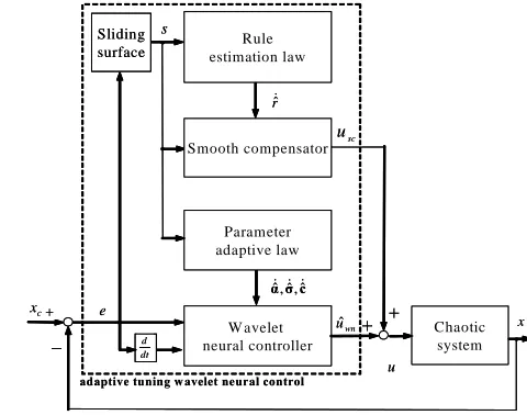
In this paper, the adaptive tuning wavelet neural control (ATWNC) system is proposed as shown in Fig. 2, where the controller output is defined as
sc
wn u
u u= ˆ +
. (14)
The wavelet neural controller uˆwn uses a WNN to approximate the ideal controller *
u , and the smooth compensator usc is utilized to compensate the approximation error between wavelet neural controller and ideal controller. The descriptions of design steps are depicted as follows:
transl at ion pro ces si ng … 1 z 2 z 1 − n z n z 1 α 2 α m α 1 Θ 2 Θ m Θ
… ∑ uwn
transl at ion pro ces si ng … 1 z 2 z 1 − n z n z 1 α 2 α m α 1 Θ 2 Θ m Θ
[image:3.595.77.261.197.304.2]… ∑ uwn
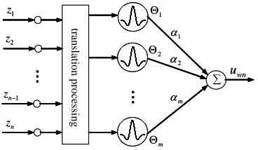
Fig. 3. Network structure of a wavelet neural network.
A. Description of WNN
The network structure of WNN is shown in Fig. 3, which can be considered as “1”-layer feedforward neural network with input preprocessing element. The WNN output with m wavelet basis functions can perform the mapping according to [9] )) ( , ( 1 j j m j j j wn
u =
∑
Θ σ z−c=
α (15)
where z T
n z z
z ]
[ 1 2K
= is the input vector, Θj(σj,(z−cj)), m
j=1,2,…, are the wavelet functions, j
σ T
nj j
j ]
[σ1 σ2 Kσ
= and cj
T nj j
jc c
c ]
[ 1 2 K
= are the
dilation and translation parameters, respectively, αj is the output layer weight. Each wavelet network’s neuron in the translation layer can be represented by
) ) ( exp( ) ( 1 2 2
∑
= − − = Θ n k kj k kj jj h z σ z c (16)
where the “Mexican hat” mother wavelet function is defined
as
∏
= − = n k k k
j w z
h 1 2 2 ) 1 ( )
(z . For ease of notation, (15) can be expressed in a compact vector form as
) , , (zσc
Θ
αT
wn
u = (17)
where T
m]
[α1α2Kα
=
α , T
m]
[Θ1Θ2 Θ
= K
Θ ,
T
m]
[σ1σ2 σ
σ= K and T
m]
[c1c2 c
c= K . This implies that there is a WNN of (17) that can uniformly approximate an ideal controller. There exists ideal weight vectors so that [9]
∆ + = * *( , *, *)
* αTΘ zσ c
u (18)
where α*
and Θ*
are optimal parameter vectors of α and
Θ, respectively; σ* and c*
are optimal parameter vectors of
σ and c, respectively; and ∆ is the approximation error. However, the optimal parameter vectors are unknown, so it is necessary to estimate the values. Define an estimation
function ) ˆ , ˆ , ( ˆ ˆ
ˆ αTΘzσc
wn
u = (19)
where αˆ and Θˆ are optimal parameter vectors of α and Θ, respectively; and σˆ and cˆ are optimal parameter vectors of
σ and c, respectively. Define the estimation error as
∆ + − = −
= ˆ α Θ αˆ Θˆ
~ * *T * T wn u u u ∆ + + +
=α~TΘ~ αˆTΘ~ α~TΘˆ
(20) where α~=α*−αˆ
and Θ~ =Θ*−Θˆ
. In order to deduce the adaptive law for mean and variance later, it is necessarily to derive the value of Θ~ . To achieve this goal, the Taylor expansion linearization technique is employed to transform the nonlinear function into a partially linear form, such that [9] h c B σ A
Θ~= T~+ T~+
(21) where σ~=σ*−σˆ
, c~=c*−cˆ
, σσ
σ σ A ˆ 1 = ⎥⎦ ⎤ ⎢⎣ ⎡ ∂ Θ ∂ ∂ Θ ∂ = m L , c c c c B ˆ 1 = ⎥⎦ ⎤ ⎢⎣ ⎡ ∂ Θ ∂ ∂ Θ ∂ = m
L , and h is the high order terms of expansion. Substitute (21) into (20), it can obtain that
∆ + + + + +
=α~ Θ~ αˆ (A σ~ B ~c h) α~ Θˆ
~ T T T T T
u ∆ + + + + +
=α~TΘˆ σ~TAαˆ ~cTBαˆ αˆTh α~TΘ~
(22) where αˆTATσ~=σ~TAαˆ
and αˆTBT~c=c~TBαˆ
are used since they are scalars. To speed up the convergence of WNN learning, the optimal parameter vector α*
is decomposed into two parts as [4]
* * * I P α α
α =ηP +ηI (23)
where ηP and ηI are positive constants, and * P α and *
I α are the proportional and integral terms of α*
, respectively, and
∫
= t d 0 * * τ P I αα . The estimation parameter vector αˆ is decomposed into two parts as
I
P α
α
αˆ=ηPˆ +ηIˆ (24)
where αˆ and P αˆ are the proportional and integral terms of I αˆ , respectively, and =
∫
t d0 ˆ ˆI αP τ
α . Thus, α~ can be expressed as * ˆ ~ ~ P P
I α α
α
α=ηI −ηP +ηP (25)
where α~I αI αˆI
*−
= . Substituting (25) into (22) obtains
Θ α α
αI ˆP P) ˆ
~ (
~ * T
P P I
u= η −η +η
∆ + + + +
+σ~TAαˆ ~cTBαˆ αˆTh ~αTΘ~ ε η
η − + + +
= α~IΘˆ αˆPΘˆ σ~ Aαˆ ~c Bαˆ T T T P T
I (26)
where the uncertain term = αPΘ+α h+α Θ+∆ ~ ~ ˆ ˆ
*T T T
P η ε . a s b s 0 PE ZO NE s (a) a s b s 0 PE ZO NE s (a) 1 r 3 r 2 r
N Z P
sc u (b) 1 r 3 r 2 r
N Z P
sc
u
(b)
[image:3.595.321.530.705.767.2]B. Smoothcompensator
Assume that the smooth compensator has 3 fuzzy rules in a rule base as given in the following form [16]
Rule 1: If s is PE, then usc is P (27) Rule 2: If s is ZO, then usc is Z (28) Rule 3: If s is NE, then usc is N (29) where the triangular-typed functions and singletons are used to define the membership functions of IF-part and THEN-part, which are depicted in Figs. 4(a) and 4(b), respectively. The defuzzification of the output is accomplished by the method of center-of-gravity
3 3 2 2 1 1 3 1 3 1 w r w r w r w w r u i i i i i
sc = = + +
∑
∑
= =
(30)
where 0≤w1≤1 , 0≤w2≤1 and0≤w3≤1 are the firing strengths of rules 1, 2, and 3, respectively; and the relation
1 3 2
1+w +w =
w is valid according to the special case of triangular membership function-based fuzzy system. In order to reduce the computation loading, let r1=rˆ, r2=0 and
r
r3=−ˆ. Hence, for any value of input x, only one of four conditions will occur according to Fig. 4(a) as [17]
Condition1: Only rule 1 is triggered ( x>xa , w1=1 , 0
3
2=w =
w )
r r
usc = 1= ˆ (31)
Condition2: Rules 1 and 2 are triggered simultaneously. (0<x≤xa, 0<w1,w2≤1 , w3=0)
1 1
1w rˆw
r
usc = = (32)
Condition3: Rules 2 and 3 are triggered simultaneously. (xb<x≤0, w1=0, 0<w2,w3≤1)
3 3
3w rˆw
r
usc = =− (33)
Condition 4: Only rule 3 is triggered. (x≤xb, w1=w2=0, 1
3=
w )
r r
usc = 3=−ˆ (34)
Then, the (31)-(34) can be rewritten as )
( ˆ w1 w3 r
usc = − (35)
Moreover, it can see that [17] 0 ) ( )
(w1−w3 = s w1−w3 ≥
s (36)
C. On-line learning algorithm
Substituting (10) into (7) and using (8), yields s u u u e k e k
e&&+ &+ = −ˆwn− sc= & *
2
1 (37)
By using the approximation property (26), (37) can be rewritten as sc T T T P T I u
s&=ηα~IΘˆ −η αˆPΘˆ +σ~ Aαˆ+~c Bαˆ+ε− . (38) To proof the stability of the ATWNC system, define a Lyapunov function candidate in the following form
c c
σ σ α
αI I
~ ~ 2 1 ~ ~ 2 1 ~ ~ 2 2
1 2 T
c T T I a s V η η η σ + + +
= (39)
where ησ and ηc are the learning rates with positive constants. Differentiating (39) with respect to time and using (38), it is obtained that
c c
σ σ α
αI&I & &
&
& ~ ~ 1 ~ ~ 1 ~T~
c T T
I
a ss
V η η η σ + + + = ) ~ ˆ ( ~ ) ~ ˆ ( ~ ) ~ ˆ ( ~ c T T T
I s s η s η
η σ c α B c σ α A σ α Θ
αI I
& &
& + + + +
+
=
) ( ˆ
ˆT sc
P s u
s + −
− η αpΘ ε (40)
If the parameter adaptive laws are selected as
Θ
αˆP=sˆ (41)
Θ α
αI I ˆ
~ ˆ =−& =s
& (42)
α
A
σ
σˆ& =−~& =ησs ˆ (43)
α
B c
cˆ&=−~& =ηcs ˆ (44)
and the smooth compensator is design as (35), then (40) can be rewritten as
=
a
V& αˆpαˆp T P η
− +s(ε−usc) ˆTˆ s rˆs(w1 w3)
P + − −
−
≤ η αpαp ε
3 1 ˆs w w r
s − −
≤ ε ) ˆ ( 3 1 3 1 w w r w w s − − − −
= ε (45)
If the following inequality
3 1 ˆ w w r −
> ε (46)
holds, then the sliding condition V&a≤0 can be satisfied. Owing to the unknown lumped uncertainties, the value rˆ cannot be exactly obtained in advance for practical applications. According to (46), there exists an ideal value *
r as follows to achieve minimum value and match the sliding condition: κ ε + − = 3 1 * w w
r (47)
where κ is a positive constant. Thus, a simple adaptive algorithm is utilized in this study to estimate the ideal value of *
r , and its estimated error is defined as r
r
r ˆ
~= *−
(48) where rˆ is the estimated value of the optimal value of *
r .
Then, define a new Lyapunov function candidate in the following form 2 2 ~ 2 1 ~ ~ 2 1 ~ ~ 2 1 ~ ~ 2 2 1 r s V r T c T T I
b η η η
η σ + + + +
= αIαI σ σ c c (49)
where ηr is the learning rate with a positive constant. Differentiating (49) with respect to time and using (38) and (41)-(44), it is obtained that
r r s s V r T c T T I
a & & & & &
& ~ ~ 1 ~ ~ 1 ~ ~ 1 ~~
η η η η σ + + + +
= αIαI σ σ c c
p pα
αˆTˆ
P η −
= s rs w w rr
r & ~ ~ 1 ) ( ˆ 1 3
η
ε− − +
+ r r w w s r s r & ~ ~ 1 ) ( ˆ 1 3
η
ε− − +
≤ r r w w s r w w s r w w s r s r & ~ ~ 1 ) ( ) ( ) (
ˆ * 1 3
3 1 * 3
1 η
ε − − + − − − +
r r w w s r w w s r s
r & ~ ~ 1 ) ( ) ( ~
3 1 * 3
1 η
ε + − − − +
=
3 1 * 3
1 ]
~ 1 ) ( [
~ sw w r s r s w w
r
r
− −
+ + −
= ε
η & (50)
Choose the rule estimation laws as )
( ˆ ~
3
1 w
w s r
r&=−&=−ηr − (51)
and using (47), (50) becomes ) ( w1 w3 s
s
V&b= ε − ε +κ −
0 3
1− ≤
−
= κs w w (52)
As a result, the stability of the proposed ATWNC system can be guaranteed.
IV. SIMULATION RESULTS
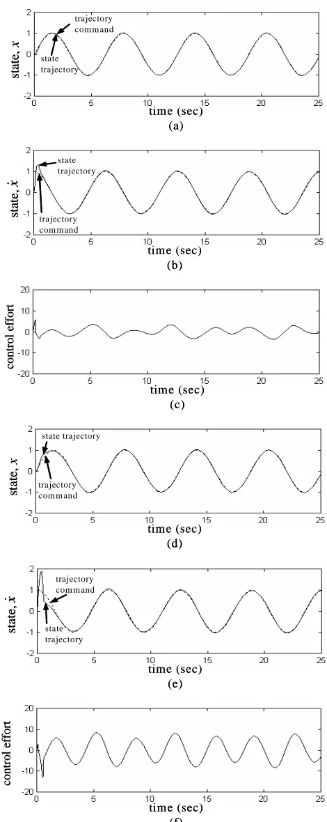
Chaotic system is a nonlinear deterministic system that displays complex, noisy-like and unpredictable behavior. It can be observed in many nonlinear circuits and mechanical systems. For control engineers, control of a chaotic system has become a significant research topic in physics, mathematics and engineering communities. The simulation results of the chaotic system are presented here to verify the effectiveness of the proposed ATWNC scheme. It should be emphasized that the derivation of ATWNC do not need to know the system dynamic function. The proposed ATWNC is applied to chaotic dynamic system again. The control parameters are selected as k1=2, k2=1, ηI=ηP=20 and
1 = =ηc
ησ . All the gains in the ATWNC are chosen to
[image:5.595.309.544.46.636.2]achieve good transient control performance in the simulation considering the requirement of stability and possible operating conditions. As ηP=0, the learning algorithm of the proposed method is the same as conventional WNN-based adaptive control. The simulation results of ATWNC with ηP =0 for q=2.1 and q=7.0 are shown in Fig. 5. The tracking responses of state
x
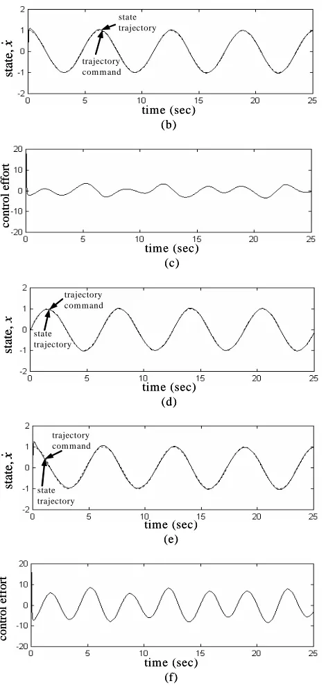
are shown in Figs. 5(a) and 5(d); the tracking responses of state x& are shown in Figs. 5(b) and 5(e); and the associated control efforts are shown Figs. 5(c) and 5(f) for q=2.1 and q=7.0 , respectively. The simulation results show that it can achieve favorable tracking performance; however, the convergence of controller parameter and tracking error is slow. Moreover, to achieve faster convergence performance, ηP=20 is reconsidered. The simulation results of ATWNC with20 = P
η for q=2.1 and q=7.0 are shown in Fig. 6. The tracking responses of state
x
are shown in Figs. 6(a) and 6(d); the tracking responses of state x& are shown in Figs. 6(b) and 6(e); and the associated control efforts are shown Figs. 6(c) and 6(f) for q=2.1 and q=7.0, respectively. From the simulation results, it is seen that the convergence of controller parameter and tracking error converge quickly.time (sec) (a)
st
at
e,
x
trajectory com m and
state trajectory
time (sec) (a)
st
at
e,
x
trajectory com m and
state trajectory
time (sec) (b)
sta
te,
x
&
trajectory com m and state trajectory
time (sec) (b)
sta
te,
x
&x
&
trajectory com m and state trajectory
time (sec) (c)
con
tro
l e
ffo
rt
time (sec) (c)
con
tro
l e
ffo
rt
time (sec) (d)
st
at
e,
x
trajectory com m and
state trajectory
time (sec) (d)
st
at
e,
x
trajectory com m and
state trajectory
time (sec) (e)
st
ate
,
x
&
trajectory comm and
state trajectory
time (sec) (e)
st
ate
,
x
&x
&
trajectory comm and
state trajectory
time (sec) (f)
con
tro
l e
ffo
rt
time (sec) (f)
con
tro
l e
ffo
rt
Fig. 5. Simulation results of ATWNC with ηP=0.
time (sec) (a)
state
,
x
trajectory comm and
state trajectory
time (sec) (a)
state
,
x
trajectory comm and
[image:5.595.317.540.677.767.2]time (sec) (b)
state,
x
&
trajectory com m and
state trajectory
time (sec) (b)
state,
x
&x
&
trajectory com m and
state trajectory
time (sec) (c)
co
n
tro
l e
ffo
rt
time (sec) (c)
co
n
tro
l e
ffo
rt
time (sec) (d)
sta
te,
x
trajectory com mand
state trajectory
time (sec) (d)
sta
te,
x
trajectory com mand
state trajectory
time (sec) (e)
state,
x
&
trajectory com mand
state trajectory
time (sec) (e)
state,
x
&x
&
trajectory com mand
state trajectory
time (sec) (f)
c
o
n
tro
l e
ffo
rt
time (sec) (f)
c
o
n
tro
l e
ffo
[image:6.595.55.290.49.545.2]rt
Fig. 6. Simulation results of ATWNC with ηP=20.
V. CONCLUSIONS
An adaptive tuning wavelet neural control (ATWNC) with a PI type learning algorithm is proposed for a chaotic dynamic system. The stability is proven by Lyapunov function with the online parameter tuning laws are given to adjust the interconnection weights, dilation and translation parameters of wavelet functions. The effectiveness of the ATWNC system is verified by some simulations. The main contributions of this paper are: (1) a learning algorithm with PI adaptation learning algorithm can achieve better tracking performance; and (2) the smooth compensator design uses a simple fuzzy system can remove completely the chattering phenomena.
ACKNOWLEDGMENT
The authors appreciate the partial financial support from the National Science Council of Republic of China under grant NSC 97-2221-E-216-029.
REFERENCES
[1] S. A. Billings and H. L. Wei, “A new class of wavelet networks for nonlinear system identification,” IEEE Trans. Neural Netw., vol. 16, no. 4, 2005, pp. 862-874.
[2] B. S. Chen and C. H. Chen, “H∞ tracking design of uncertain nonlinear SISO systems: adaptive fuzzy approach,” IEEE Trans. Fuzzy Syst., vol. 4, no. 1, 1996, pp. 32-43.
[3] G. Chen and X. Dong, “On Feedback Control of Chaotic Continuous-Time Systems,” IEEE Trans.Circuits Syst. I, vol. 40, no. 9, 1993, pp. 591-601.
[4] N. Golea, A. Golea, and K. Benmahammed, “Fuzzy model reference adaptive control,” IEEE Trans. Fuzzy Syst., vol. 10, no. 4, 2002, pp. 436-444.
[5] C. F. Hsu, C. M. Lin, and T. Y. Chen, “Neural-network-identification-based adaptive control of wing rock motion,” IEE Proc., Contr. Theory Appl., vol. 152, no.1, 2005, pp. 65-71.
[6] C. F. Hsu, C. M. Lin, and T. T. Lee, “Wavelet adaptive backstepping control for a class of nonlinear systems,” IEEE Trans. Neural Netw., vol. 17, no. 5, 2006, pp. 1175-1183.
[7] J. Q. Huang and F. L. Lewis, “Neural-network predictive control for nonlinear dynamic systems with time-delay,” IEEE Trans. Neural Netw., vol. 14, no. 2, 2003, pp. 377-389.
[8] Z. P. Jiang, “Advanced feedback control of the chaotic Duffing equation,” IEEE Trans. Circuits Syst. I, vol. 49, no. 2, 2002, pp. 244-249.
[9] C. K. Lin, “Adaptive tracking controller design for robotic systems using Gaussian wavelet networks,” IEE Proc., Contr. Theory Appl., vol. 149, no. 4, 2002, pp. 316-322.
[10] C. M. Lin and C. F. Hsu, “Neural network hybrid control for antilock braking systems,” IEEE Trans. Neural Netw., vol. 14, no. 2, 2003, pp. 351-359.
[11] A. Loría and A. Zavala-Río, “Adaptive tracking control of chaotic systems with applications to synchronization,” IEEE Trans. Circuits Syst., I, vol. 54, no. 9, 2007, pp. 2019-2029.
[12] O. Omidvar and D. L. Elliott, Neural Systems for Control, Academic Press 1997.
[13] J. H. Park, S. J. Seo, and G. T. Park, “Robust adaptive fuzzy controller for nonlinear system using estimation of bounds for approximation errors,” Fuzzy Set Syst., vol. 133, no. 1, 2003, pp. 19-36.
[14] J. J. E. Slotine and W. P. Li, Applied Nonlinear Control, Englewood Cliffs, NJ: Prentice Hall, 1991.
[15] C. D. Sousa, E. M. Hemerly, and R. K. H. Galvao, “Adaptive control for mobile robot using wavelet networks,” IEEE Trans. Syst., Man and Cybern.,Pt B, vol. 32, no. 4, 2002, pp. 493-504.
[16] J. R. Timothy, Fuzzy Logic with Engineering Application. NewYork: Mc-Graw Hill, 1995.
[17] R. J. Wai, “Fuzzy sliding-mode control using adaptive tuning technique,” IEEE Trans. Industrial Electronics, vol. 54, no. 1, 2007, pp. 586-594.
[18] H. Wang and Y. Wang, “Neural-network-based fault-tolerant control of unknown nonlinear systems,” IEE Proc., Contr. Theory Appl., vol. 146, no. 5, 1999, pp. 389-398.
[19] W. Y. Wang, M. L. Chan, C. C. J. Hsu, and T. T. Lee, “H∞
tracking-based sliding mode control for uncertain nonlinear systems via an adaptive fuzzy-neural approach,” IEEE Trans. Syst., Man and Cybern.,Pt B, vol. 32, no. 4, 2002, pp. 483-492.