Bayesian Checking for Topic Models

Proceedings of the 2011 Conference on Empirical Methods in Natural Language Processing, pages 227–237,

Bayesian Checking for Topic Models

David Mimno

Department of Computer Science Princeton University Princeton, NJ 08540

mimno@cs.princeton.edu

David Blei

Department of Computer Science Princeton University Princeton, NJ 08540

blei@cs.princeton.edu

Abstract

Real document collections do not fit the inde-pendence assumptions asserted by most statis-tical topic models, but how badly do they vi-olate them? We present a Bayesian method for measuring how well a topic model fits a corpus. Our approach is based on posterior predictive checking, a method for diagnosing Bayesian models in user-defined ways. Our method can identify where a topic model fits the data, where it falls short, and in which di-rections it might be improved.

1 Introduction

Probabilistic topic models are a suite of machine learning algorithms that decompose a corpus into a set of topics and represent each document with a subset of those topics. The inferred topics often cor-respond with the underlying themes of the analyzed collection, and the topic modeling algorithm orga-nizes the documents according to those themes.

Most topic models are evaluated by their predic-tive performance on held out data. The idea is that topic models are fit to maximize the likelihood (or posterior probability) of a collection of documents, and so a good model is one that assigns high likeli-hood to a held out set (Blei et al., 2003; Wallach et al., 2009).

But this evaluation is not in line with how topic models are frequently used. Topic mod-els seem to capture the underlying themes of a collection—indeed the monicker “topic model” is retrospective—and so we expect that these themes are useful for exploring, summarizing, and learning

about its documents (Mimno and McCallum, 2007; Chang et al., 2009). In such exploratory data anal-ysis, however, we are not concerned with the fit to held out data.

In this paper, we develop and study new methods for evaluating topic models. Our methods are based on posterior predictive checking, which is a model diagnosis technique from Bayesian statistics (Rubin, 1984; Gelman et al., 1996). The goal of a posterior predictive check (PPC) is to assess the validity of a Bayesian model without requiring a specific alterna-tive model. Given data, we first compute a posterior distribution over the latent variables. Then, we esti-mate the probability of the observed data under the data-generating distribution that is induced by the posterior (the “posterior predictive distribution”). A data set that is unlikely calls the model into ques-tion, and consequently the posterior. PPCs can show where the model fits and doesn’t fit the observations. They can help identify the parts of the posterior that are worth exploring.

The key to a posterior predictive check is the dis-crepancy function. This is a function of the data that measures a property of the model which is impor-tant to capture. While the model is often chosen for computational reasons, the discrepancy function might capture aspects of the data that are desirable but difficult to model. In this work, we will design a discrepancy function to measure an independence assumption that is implicit in the modeling assump-tions but is not enforced in the posterior. We will embed this function in a posterior predictive check and use it to evaluate and visualize topic models in new ways.

Specifically, we develop discrepancy functions for latent Dirichlet allocation (the simplest topic model) that measure how well its statistical assump-tions about the topics are matched in the observed corpus and inferred topics. LDA assumes that each observed word in a corpus is assigned to a topic, and that the words assigned to the same topic are drawn independently from the same multinomial distribu-tion (Blei et al., 2003). For each topic, we mea-sure the whether this assumption holds by comput-ing the mutual information between the words as-signed to that topic and which document each word appeared in. If the assumptions hold, these two vari-ables should be independent: low mutual informa-tion indicates that the assumpinforma-tions hold; high mu-tual information indicates a mismatch to the model-ing assumptions.

We embed this discrepancy in a PPC and study it in several ways. First, we focus on topics that model their observations well; this helps separate interpretable topics from noisy topics (and “boiler-plate” topics, which exhibit too little noise). Sec-ond, we focus on individual terms within topics; this helps display a model applied to a corpus, and under-stand which terms are modeled well. Third, we re-place the document identity with an external variable that might plausibly be incorporated into the model (such as time stamp or author). This helps point the modeler towards the most promising among more complicated models, or save the effort in fitting one. Finally, we validate this strategy by simulating data from a topic model, and assessing whether the PPC “accepts” the resulting data.

2 Probabilistic Topic Modeling

Probabilistic topic models are statistical models of text that assume that a small number of distributions over words, called “topics,” are used to generate the observed documents. One of the simplest topic mod-els is latent Dirichlet allocation (LDA) (Blei et al., 2003). In LDA, a set of K topics describes a

cor-pus; each document exhibits the topics with different proportions. The words are assumed exchangeable within each document; the documents are assumed exchangeable within the corpus.

More formally, letφ1, . . . , φK beK topics, each

of which is a distribution over a fixed vocabulary.

For each document, LDA assumes the following generative process

1. Choose topic proportionsθd∼Dirichlet(α).

2. For each word

(a) Choose topic assignmentzd,n∼θ.

(b) Choose wordwd,n∼φzd,n.

This process articulates the statistical assumptions behind LDA: Each document is endowed with its own set of topic proportionsθd, but the same set of

topicsφ1:Kgoverns the whole collection.

Notice that the probability of a word is indepen-dent of its document θd given its topic assignment

zd,n (i.e.,wd,n ⊥⊥ θd|zd,n). Two documents might

have different overall probabilities of containing a word from the “vegetables” topic; however, all the words in the collection (regardless of their docu-ments) drawn from that topic will be drawn from the same multinomial distribution.

The central computational problem for LDA is posterior inference. Given a collection of docu-ments, the problem is to compute the conditional distribution of the hidden variables—the topicsφk,

topic proportions θd, and topic assignments zd,n.

Researchers have developed many algorithms for approximating this posterior, including sampling methods (Griffiths and Steyvers, 2004) (used in this paper), variational methods (Blei et al., 2003), dis-tributed variants (Asuncion et al., 2008), and online algorithms (Hoffman et al., 2010).

3 Checking Topic Models

Once approximated, the posterior distribution is used for the task at hand. Topic models have been applied to many tasks, such as classification, predic-tion, collaborative filtering, and others. We focus on using them as an exploratory tool, where we as-sume that the topic model posterior provides a good decomposition of the corpus and that the topics pro-vide good summaries of the corpus contents.

Score Rank 14 12 10 8 6 4 2 14 12 10 8 6 4 2 14 12 10 8 6 4 2 Topic850 weekend Broadway Times listing selective noteworthy critics tickets highly recommended denotes booth Tickets Street TKTS Topic628 Iraq Iraqi Hussein Baghdad Saddam Shiite government al Iraqis Sunni Kurdish forces country military troops Topic87 Roberts Grant Fort Worth Burke Hunt Kravis Bass Kohlberg Grace Rothschild Baron Borden Texas William

1 2 3 4

Topic371 Tickets Through Street Road Saturdays Sundays New Fridays Jersey Hours Free Tuesdays MUSEUM Thursdays THEATER Topic178 agency safety report Federal Administration problems investigation Safety violations federal failed inspector review department general Topic750 Four Freeman Seasons Da Vinci Code Thomson Wolff Leonardo Brown Three Dan Cliff Holy da

1 2 3 4

Topic760 Week book Warner sales List Weeks woman bookstores death indicates Advice Putnam OF report New Topic632 job jobs working office business career worked employees hired boss manager find corporate help experience Topic274 Leon Levy Hess Bard LEVY Botstein Atlas Shelby Panetta Norman Wieseltier HESS David Amerada Norma

1 2 3 4

Figure 1:Visualization of variability within topics. Nine randomly selected topics from the New York Times with low (top row), medium (middle row) and high (bottom row) mutual information between words and documents. The

intuition is that only when satisfied with the model should the modeler use the posterior to learn about her data. In complicated Bayesian models, such as topic models, Bayesian model checking can point to the parts of the posterior that better fit the observed data set and are more likely to suggest something meaningful about it.

In particular, we will develop posterior predictive checks (PPC) for topic models. In a PPC, we spec-ify a discrepancy function, which is a function of the data that measures an important property that we want the model to capture. We then assess whether the observed value of the function is similar to val-ues of the function drawn from the posterior, through the distribution of the data that it induces. (This dis-tribution of the data is called the “posterior predic-tive distribution.”)

An innovation in PPCs is therealized discrepancy function(Gelman et al., 1996), which is a function of the data and any hidden variables that are in the model. Realized discrepancies induce a traditional discrepancy by marginalizing out the hidden vari-ables. But they can also be used to evaluate assump-tions about latent variables in the posterior, espe-cially when combined with techniques like MCMC sampling that provide realizations of them. In topic models, as we will see below, we use a realized dis-crepancy to factor the observations and to check spe-cific components of the model that are discovered by the posterior.

3.1 A realized discrepancy for LDA

Returning to LDA, we design a discrepancy func-tion that checks the independence assumpfunc-tion of words given their topic assignments. As we men-tioned above, given the topic assignmentzthe word w should be independent of its document θ.

Con-sider a decomposition of a corpus from LDA, which assigns every observed word wd,n to a topic zd,n.

Now restrict attention to all the words assigned to the

kth topic and form two random variables:W are the

words assigned to the topic andDare the document

indices of the words assigned to that topic. If the LDA assumptions hold then knowing W gives no

information about D because the words are drawn independently from the topic.

We measure this independence with the mutual

information betweenW andD:1

M I(W, D|k)

=X

w

X

d

P(w, d_|k) logP(w|d, k)P(d|k)

P(w_|k)P(d_|k)

=X

w

X

d

N(w, d, k)

N(k) log

N(w, d, k)N(k)

N(d, k)N(w, k). (1)

WhereN(w, d, k) is the number of tokens of type

w in topic k in document d, with N(w, k) =

P

dN(w, d, k), N(d, k) =

P

wN(w, d, k), and

N(k) = P_w,dN(w, d, k). This function mea-sures the divergence between the joint distribution over word and document index and the product of the marginal distributions. In the limit of infinite samples, independent random variables have mutual information of zero, but we expect finite samples to have non-zero values even for truly independent variables. Notice that this is a realized discrepancy; it depends on the latent assignments of observed words to topics.

Eq. 1 is defined as a sum over a set of documents and a set of words. We can rearrange this summa-tion as a weighted sum of theinstantaneous mutual informationbetween words and documents:

IM I(w, D_|k) =H(D_|k)₋H(D_|W =w, k).

(2) This quantity can be understood by considering the per-topic distribution of document labels, p(d_|k).

This distribution is formed by normalizing the counts of how many words assigned to topick

ap-peared in each document. The first term of Eq. 2 is the entropy—some topics are evenly distributed across many documents (high entropy); others are concentrated in fewer documents (low entropy).

The second term conditions this distribution on a particular word type w by normalizing the

per-document number of timeswappeared in each

doc-ument (in topic k). If this distribution is close

to p(d_|k) then H(D_|W = w, k) will be close to

H(D|k)and IM I(w, D|k)will be low. If, on the

other hand, wordwoccurs many times in only a few

documents, it will have lower entropy over

docu-1_{There are other choices of discrepancies, such as}

ments than the overall distribution over documents for the topic andIM I(w, D_|k)will be high.

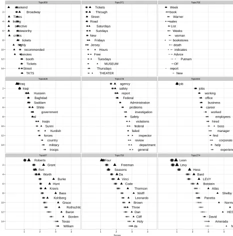
We illustrate this discrepancy in Figure 1, which shows nine topics trained from theNew York Times.2

Each row contains randomly selected topics from low, middle, and high ranges of MI, respectively. Each triangle represents a word. Its place on they

-axis is its rank in the topic. Its place on thex-axis

is its IM I(w_|k), with more uniformly distributed

words (low IMI) to the left and more specific words (high IMI) to the right. (For now, ignore the other points in this figure.) IMI varies between topics, but tends to increase with rank as less frequent words appear in fewer documents.

The discrepancy captures different kinds of struc-ture in the topics. The top left topic represents for-mulaic language, language that occurs verbatim in many documents. In particular, it models the boil-erplate text “Here is a selective listing by critics of The Times of new or noteworthy...” Identifying re-peated phrases is a common phenomenon in topic models. Most words show lower than expected IMI, indicating that word use in this topic is less vari-able than data drawn from a multinomial distribu-tion. The middle-left topic is an example of a good topic, according to this discrepancy, which is related to Iraqi politics. The bottom-left topic is an example of the opposite extreme from the top-left. It shows a loosely connected series of proper names with no overall theme.

3.2 Posterior Predictive Checks for LDA

Intuitively, the middle row of topics in Figure 1 are the sort of topics we look for in a model, while the top and bottom rows contain topics that are less use-ful. Using a PPC, we can formally measure the dif-ference between these topics. For each of the real topics in Figure 1 we regenerated the same figure 20 times. We sampled new words for every token from the posterior distribution of the topic, and re-calculated the rank and IMI for each word. These “shadow” figures are shown as gray circles. The density of those circles creates a reference distribu-tion indicating the expected IMI values at each rank under the multinomial assumption.

2_{Details about the corpus and model fitting are in Section}

4.2. Similar figures for two other corpora are in the supplement.

By themselves, IMI scores give an indication of the distribution of a word between documents within a topic: small numbers are better, large numbers in-dicate greater discrepancy. These scores, however, are based on the specific allocation of words to top-ics. For example, lower-ranked, less frequent words within a topic tend to have higher IMI scores than higher-ranked, more frequent words. This difference may be due to greater violation of multinomial as-sumptions, but may also simply be due to smaller sample sizes, as the entropyH(D_|W =w, k)is es-timated from fewer tokens. The reference distribu-tions help distinguish between these two cases.

In more detail, we generate replications of the data by considering a Gibbs sampling state. This state assigns each observed word to a topic. We first record the number of instances of each term as-signed to each topic,N(w|k). Then for each word

wd,nin the corpus, we sample a new observed word

wrep_d,n whereP(w) _∝ N(w_|zd,n). (We did not use

smoothing parameters.) Finally, we recalculate the mutual information and instantenous mutual infor-mation for each topic.

In the top-left topic, most of the words have much lower IMI than the word at the same rank in repli-cations, indicating lower than expected variability. The exception is the wordBroadway, which is more variable than expected. In the middle-left topic, IMI for the wordsIraqi andBaghdad occur within the expected range. These words fit the multino-mial assumption: any word assigned to this topic is equally likely to beIraqi. Values for the words

Shiite,Sunni, andKurdish are more specific to par-ticular documents than we expect under the model. In the bottom-left topic, almost all words occur with greater variability than expected. This topic com-bines many terms with only coincidental similarity, such as Mets pitcher Grant Roberts and the firm Kohlberg Kravis Roberts.

Deviance

count

0 5 10 15 20 25 30

0 5 10 15 20 25 30

0 5 10 15 20 25 30

Topic850

Topic628

Topic87

−20 0 20 40

Figure 2:News: Observed topic scores (vertical lines) relative to replicated scores, rescaled so that replica-tions have zero mean and unit variance.TheWeekend topic (top) has lower than expected MI. TheIraq (mid-dle) and Roberts (bottom) topics both have MI greater than expected.

and Roberts topics have significantly greater than expected MI.

For most topics the actual discrepancy is outside the range of any replicated discrepancies. In their original formulation, PPCs prescribe computing a tail probability of a replicated discrepancy being greater than (or less than) the observed discrepancy under the posterior predictive distribution. For ex-ample if an observed value is greater than 70 of 100 replicated values, we report a PPCp-value of 0.7.

When the observed value is far outside the range of any replicated values, as in Figure 2, that tail probability will be degenerate at 0 or 1. So, we re-port instead adeviancevalue, an alternative way of comparing an observed value to a reference distri-bution. We compute the distribution of the repli-cated discrepancies and compute its standard devi-ation. We then compute how many standard devia-tions the observed discrepancy is from the mean of the replicated discrepancies.

This score allows us to compare topics. The ob-served value for theWeekendtopic is 31.8 standard deviations below the mean replicated value, and thus has deviance of -31.8, which is lower than expected. TheIraqtopic has deviance of 16.8 and theRoberts

topic has deviance of 47.7. This matches our intu-ition that the former topic is more useful than the latter.

4 Searching for Systematic Deviations We demonstrated that the mutual information dis-crepancy function can detect violations of multi-nomial assumptions, in which instances of a term in a given topic are not independently distributed among documents. One way to address this lack of fit is to encode document-level extra-multinomial variance (“burstiness”) into the model using Dirich-let compound multinomial distributions (Doyle and Elkan, 2009). If there is no pattern to the deviations from multinomial word use across documents, this method is the best we can do.

In many corpora, however, there are systematic deviations that can be explained by additional vari-ables. LDA is the simplest generative topic model, and researchers have developed many variants of LDA that account for a variety of variables that can be found or measured with a corpus. Examples in-clude models that account for time (Blei and Laf-ferty, 2006), books (Mimno and McCallum, 2007), and aspect or perspective (Mei and Zhai, 2006; Lin et al., 2008; Paul et al., 2010). In this section, we show how we can use the mutual information dis-crepancy function of Equation 1 and PPCs to guide our choice in which topic model to fit.

Greater deviance implies that a particular group-ing better explains the variation in word use within a topic. The discrepancy functions are large when words appear more than expected in some groups and less than expected in others. We know that the individual documents show significantly more variation than we expect from replications from the model’s posterior distribution. If we combine docu-ments randomly in a meaningless grouping, such de-viance should decrease, as differences between doc-uments are “smoothed out.” If a grouping of docu-ments shows equal or greater deviation, we can as-sume that that grouping is maintaining the underly-ing structure of the systematic deviation from the multinomial assumption, and that further modeling or visualization using that grouping might be useful.

4.1 PPCs for systematic discrepancy

Score

Rank

20 15 10 5

Documents

Iraq Iraqi

Hussein Baghdad Saddam

Shiite government al

Iraqis Sunni

Kurdish forces

country military

troops leaders city

Kurds security

Sadr

0.0 0.5 1.0 1.5 2.0 2.5

Months

Iraq Iraqi

Hussein Baghdad Saddam

Shiite government al

Iraqis Sunni Kurdish forces country

military troops leaders city

Kurds security

Sadr

0.0 0.5 1.0 1.5 2.0 2.5

Desks

Iraq Iraqi Hussein

Baghdad Saddam

Shiite government al

Iraqis Sunni

Kurdish forces country military troops

leaders city Kurds

security Sadr

0.0 0.5 1.0 1.5 2.0 2.5

Figure 3: Groupings decrease MI, but values are still larger than expected. Three ways of grouping words in a topic from theNew York Times. The wordleadersvaries more between desks than by time, whileSadrvaries more by time than desk.

variablegin the discrepancy. For example, the New York Times articles are each associated with a par-ticular news desk and also associated with a time stamp. If the topic modeling assumptions hold, the words are independent of both these variables. If we see a significant discrepancy relative to a grouping defined by a metadata feature, this systematic vari-ability suggests that we might want to take that fea-ture into account in the model.

Let G be a set of groups and let γ ∈ GD _be

a grouping of D documents. Let N(w, g, k) =

P

dN(w, d, k)Iγd=g, that is, the number of words of

typewin topickin documents in groupg, and define

the other count variables similarly. We can now sub-stitute these group-specific counts for the document-specific counts in the discrepancy function in Eq. 1. Note that the previous discrepancy functions are equivalent to a trivial grouping, in which each docu-ment is the only member of its own group. In the fol-lowing experiments we explore groupings by pub-lished volume, blog, preferred political candidate, and newspaper desk, and evaluate the effect of those groupings on the deviation between mean replicated values and observed values of those functions.

4.2 Case studies

We analyze three corpora, each with its own meta-data: the New York Times Annotated Corpus (1987– 2007)3_{, the CMU 2008 political blog corpus}

(Eisen-stein and Xing, 2010), and speeches from the British

3_{http://www.ldc.upenn.edu}

House of Commons from 1830–1891.4 _Descriptive

statistics are presented in Table 1. The realization is represented by a single Gibbs sampling state after 1000 iterations of Gibbs sampling.

Table 1: Statistics for models used as examples. Name Docs Tokens Vocab Topics

News 1.8M 76M 121k 1000

Blogs 13k 2.2M 90k 100

Parliament 540k 55M 52k 300

New York Times articles. Figure 3 shows three groupings of words for the middle-left topic in Fig-ure 1: by document, by month of publication (e.g. May of 2005), and by desk (e.g. Editorial, Foreign, Financial). Instantaneous mutual information values are significantly smaller for the larger groupings, but the actual values are still larger than expected under the model. We are interested in measuring the de-gree to which word usage varies within topics as a function of both time and the perspective of the ar-ticle. For example, we may expect that word choice may differ between opinion articles, which overtly reflect an author’s views, and news articles, which take a more objective, factual approach.

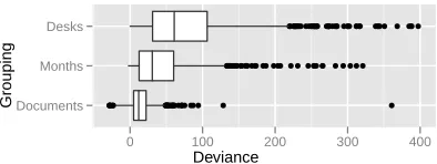
We summarize each grouping by plotting the dis-tribution of deviance scores for all topics. Results for all 1000 topics grouped by documents, months, and desks are shown in Figure 4.

Deviance

GroupingDocuments

Months Desks

● ●●●● ●

●● ●●● ●

●● ●●●●● ●●●●●●●●● ●●● ● ● ●

● ● ● ●● ● ●●●● ●●●●● ●●●●●

●● ●

●● ●

● ● ●

● ● ●

●● ●●●●● ● ●● ●●● ●● ● ● ● ● ●● ●●●●●●●●●● ●●●● ●●● ●● ●●● ●● ●● ●● ● ●● ● ●●● ● ● ●

0 100 200 300 400

Figure 4:News: Lack of fit correlates best with desks.

We calculate the number of standard deviations between the mean replicated discrepancy and the actual discrep-ancy for each topic under three groupings. Boxes repre-sent typical ranges, points reprerepre-sent outliers.

Month

Score

0.0000 0.0005 0.0010 0.0015

0.0000 0.0005 0.0010 0.0015

0e+00 2e−04 4e−04 6e−04

0.0000 0.0005 0.0010 0.0015 0.0020 0.0025

0e+00 2e−04 4e−04 6e−04 8e−04

−2e−040e+00

2e−04 4e−04 6e−04

Kurdish

Hussein

Sunni

Sadr

Maliki

Shiite

1987 1992 1997 2002 2007

Figure 5: News: Events change word distributions.

Words with the largest MI from a topic on Iraq’s gov-ernment are shown, with individual scores grouped by month.

Finally, we can analyze how individual words in-teract with groupings like time or desk. Figure 5 breaks down the per-word discrepancy shown in Fig-ure 3 by month, for the words with the largest overall discrepancy. Kurdish is prominent during the Gulf War and the 1996 cruise missile strikes, but is less significant during the Iraq War. Individuals ( Hus-sein,Sadr, andMaliki) move on and off the stage.

Political blogs. The CMU 2008 political blog cor-pus consists of six blogs, three of which supported Barack Obama and three of which supported John McCain. This corpus has previously been consid-ered in the context of aspect-based topic models (Ahmed and Xing, 2010) that assign distinct word distributions to liberal and conservative bloggers. It is reasonable to expect that blogs with different po-litical leanings will use measurably different lan-guage to describe the same themes, suggesting that there will be systematic deviations from a multino-mial hypothesis of exchangeability of words within topics. Indeed, Ahmed and Xing obtained improved results with such a model. Figure 6 shows the dis-tribution of standard deviations from the mean repli-cated value for a set of 150 topics grouped by doc-ument, blog, and preferred candidate. Deviance is greatest for blogs, followed by candidates and then documents.

Deviance

GroupingDocuments

Blogs Candidates

●

●● ●●

● ●

● ●● ●

0 100 200 300 400

Figure 6:Blogs: Lack of fit correlates more with blog than preferred candidate. Grouping by preferred can-didate has only slightly higher average deviance than by documents, but the variance is greater.

two candidates. To determine whether this particular assignment of documents to blogs is responsible for the difference in discrepancy functions or whether any such split would have greater deviance, we com-pared random groupings to the real groupings and recalculate the PPC. We generated 10 such group-ings by permuting document blog labels and another 10 by permuting document candidate labels, each time holding the topics fixed. The average number of standard deviations across topics was6.6_±14.4

for permuted “candidates” compared to37.9_±39.2

for the real corpus, and 10.6±12.9 for permuted

“blogs” compared to44.4_±29.6for real blogs.

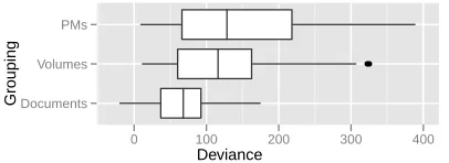
British parliament proceedings. The parliament corpus is divided into 305 volumes, each comprising about three weeks of debates, with between 600 and 4000 speeches per session. In addition to volumes, 10 Prime Ministers were in office during this period.

Deviance

GroupingDocuments

Volumes PMs

● ●

0 100 200 300 400

Figure 7:Parliament: Lack-of-fit correlates with time (publication volume). Correlation with prime ministers is not significantly better than with volume.

Grouping by prime minister shows greater av-erage deviance than grouping by volumes, even though there are substantially fewer divisions. Al-though such results would need to be accompanied by permutation experiments as in the blog corpus, this methodology may be of interest to historians.

In order to provide insight into the nature of tem-poral variation, we can group the terms in the sum-mation in Equation 1 by word and rank the words by their contribution to the discrepancy function. Fig-ure 8 shows the most “mismatching” words for a topic with the most probable words ships, vessels, admiralty, iron, ship, navy, consistent with changes in naval technology during the Victorian era (that is, wooden ships to “iron clads”). Words that oc-cur more prominently in the topic (ships, vessels) are also variable, but more consistent across time.

Volume

Score

0.0000 0.0005 0.0010 0.0015

0.0000 0.0005 0.0010 0.0015

0.0000 0.0005 0.0010 0.0015

0.0000 0.0005 0.0010 0.0015

0.0000 0.0005 0.0010 0.0015

0.0000 0.0005 0.0010 0.0015

iron

turret

clads

wooden

vessels

ships

1830 1835 1840 1845 1850 1855 1860 1865 1870 1875 1880 1885 1890

Figure 8: Parliament: iron-cladsintroduced in 1860s.

High probability words (ships, vessels) are variable, but show less concentrated discrepancy thaniron, wooden.

5 Calibration on Synthetic Data

A posterior predictive check asks “do observations sampled from the learned model look like the origi-nal data?” In the previous sections, we have consid-ered PPCs that explore variability within a topic on a per-word basis, measure discrepancy at the topic level, and compare deviance over all topics between groupings of documents. Those results show that the PPC detects deviation from multinomial assump-tions when it exists: as expected, variability in word choice aligns with known divisions in corpora, for example by time and author perspective. We now consider the opposite direction. When documents are generated from a multinomial topic model, PPCs should not detect systematic deviation.

We must also distinguish between lack of fit due to model misspecification and lack of fit due to ap-proximate inference. In this section, we present syn-thetic data experiments where the learned model is precisely the model used to generate documents. We show that there is significant lack of fit introduced by approximate inference, which can be corrected by considering only parts of the model that are well-estimated.

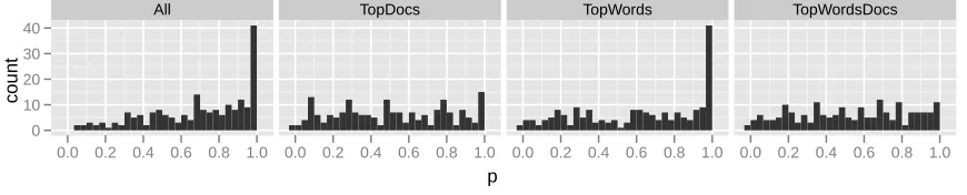
p

count

0 10 20 30 40

All

0.0 0.2 0.4 0.6 0.8 1.0

TopDocs

0.0 0.2 0.4 0.6 0.8 1.0

TopWords

0.0 0.2 0.4 0.6 0.8 1.0

TopWordsDocs

0.0 0.2 0.4 0.6 0.8 1.0

Figure 9:Replicating only documents with large allocation in the topic leads to more uniformp-values.p-values

for 200 topics estimated from synthetic data generated from an LDA model are either uniform or skewed towards 1.0. Overly conservativep-values would be clustered around 0.5.

topics over a vocabulary of 100 terms. Hyperpa-rameters for both the document-topic and topic-term Dirichlet priors were 0.1 for each dimension. We then trained a topic model with the same hyperpa-rameters and number of topics on each corpus, sav-ing a Gibbs samplsav-ing state.

We can measure the fit of a PPC by examining the distribution of empiricalp-values, that is, the

propor-tion of replicapropor-tionswrep that result in discrepancies less than the observed value.p-values should be

uni-formly distributed on(0,1). Non-uniformp-values

indicate a lack of calibration. Unlike real collec-tions, in synthetic corpora the range of discrepan-cies from these replicated collections often includes the real values, sop-values are meaningful. A

his-togram ofp-values for 200 synthetic topics after 100

replications is shown in the left panel of Figure 9. PPCs have been criticized for reusing training data for model checking. For some models, the posterior distribution is too close to the data, so all replicated values are close to the real value, leading to p-values clustered around 0.5 (Draper and

Krn-jajic, 2006; Bayarri and Castellanos, 2007). We test divergence from a uniform distribution with a Kolmogorov-Smirnov test. Our results indicate that LDA is not overfitting, but that the distribution is not uniform (KSp <0.00001).

The PPC framework allows us to choose discrep-ancy functions that reflect the relative importance of subsets of words and documents. The second panel in Figure 9 sums only over the 20 documents with the largest probability of the topic, the third sums over all documents but only over the top 10 most probable words, and the fourth sums over only the top words and documents. This test indicates

that the distribution ofp-values for the subset Top-Wordsis not uniform (KSp < 0.00001), but that a

uniform distribution is a good fit forTopDocs (KS

p= 0.358) andTopWordsDocs(KSp= 0.069).

6 Conclusions

We have developed a Bayesian model checking method for probabilistic topic models. Conditioned on their topic assignment, the words of the docu-ments are independently and identically distributed by a multinomial distribution. We developed a real-ized discrepancy function—the mutual information between words and document indices, conditioned on a topic—that checks this assumption. We em-bedded this function in a posterior predictive check. We demonstrated that we can use this posterior predictive check to identify particular topics that fit the data, and particular topics that misfit the data in different ways. Moreover, our method provides a new way to visualize topic models.

We adapted the method to corpora with external variables. In this setting, the PPC provides a way to guide the modeler in searching through more com-plicated models that involve more variables.

Finally, on simulated data, we demonstrated that PPCs with the mutual information discrepancy func-tion can identify model fit and model misfit.

Acknowledgments

Eggers suggested the use of the Hansards corpus.

References

Amr Ahmed and Eric Xing. 2010. Staying informed: Su-pervised and semi-suSu-pervised multi-view topical anal-ysis of ideological perspective. InEMNLP.

Arthur Asuncion, Padhraic Smyth, and Max Welling. 2008. Asynchronous distributed learning of topic models. InNIPS.

M.J. Bayarri and M.E. Castellanos. 2007. Bayesian checking of the second levels of hierarchical models. Statistical Science, 22(3):322–343.

David M. Blei and John D. Lafferty. 2006. Dynamic topic models. InICML.

David Blei, Andrew Ng, and Michael Jordan. 2003. La-tent Dirichlet allocation. Journal of Machine Learning Research, 3:993–1022, January.

Jonathan Chang, Jordan Boyd-Graber, Chong Wang, Sean Gerrish, and David M. Blei. 2009. Reading tea leaves: How humans interpret topic models. In Ad-vances in Neural Information Processing Systems 22, pages 288–296.

Gabriel Doyle and Charles Elkan. 2009. Accounting for burstiness in topic models. InICML.

David Draper and Milovan Krnjajic. 2006. Bayesian model specification. Technical report, University of California, Santa Cruz.

Jacob Eisenstein and Eric Xing. 2010. The CMU 2008 political blog corpus. Technical report, Carnegie Mel-lon University.

A. Gelman, X.L. Meng, and H.S. Stern. 1996. poste-rior predictive assessment of model fitness via realized discrepancies. Statistica Sinica, 6:733–807.

Thomas L. Griffiths and Mark Steyvers. 2004. Finding scientific topics. PNAS, 101(suppl. 1):5228–5235. Matthew Hoffman, David Blei, and Francis Bach. 2010.

Online learning for latent dirichlet allocation. InNIPS. Wei-Hao Lin, Eric Xing, and Alexander Hauptmann. 2008. A joint topic and perspective model for ideo-logical discourse. InPKDD.

Qiaozhu Mei and ChengXiang Zhai. 2006. A mixture model for contextual text mining. InKDD.

David Mimno and Andrew McCallum. 2007. Organizing the OCA: learning faceted subjects from a library of digital books. InJCDL.

David Newman, Jey Han Lau, Karl Grieser, and Timothy Baldwin. 2010. Automatic evaluation of topic coher-ence. InHuman Language Technologies: The Annual Conference of the North American Chapter of the As-sociation for Computational Linguistics.

Michael J. Paul, ChengXiang Zhai, and Roxana Girju. 2010. Summarizing contrastive viewpoints in opin-ionated text. InEMNLP.

Donald B. Rubin. 1981. Estimation in parallel random-ized experiments. Journal of Educational Statistics, 6:377–401.

D. Rubin. 1984. Bayesianly justifiable and relevant fre-quency calculations for the applied statistician. The Annals of Statistics, 12(4):1151–1172.