Analyzing Correlated Evolution of Multiple Features
Using Latent Representations
Yugo Murawaki
Graduate School of Informatics, Kyoto University Yoshida-honmachi, Sakyo-ku, Kyoto, 606-8501, Japan
Abstract
Statistical phylogenetic models have allowed the quantitative analysis of the evolution of a single categorical feature and a pair of binary features, but correlated evolution involving multiple discrete features is yet to be explored. Here we propose latent representation-based analysis in which (1) a sequence of discrete surface features is projected to a sequence of independent binary variables and (2) phylo-genetic inference is performed on the latent space. In the experiments, we analyze the fea-tures of linguistic typology, with a special fo-cus on the order of subject, object and verb. Our analysis suggests that languages sharing the same word order are not necessarily a co-herent group but exhibit varying degrees of di-achronic stability depending on other features.
1 Introduction
Research on structural properties (typological fea-tures) of language, such as the order of subject, ob-ject and verb (examples areSOVandSVO) and the presence or absence of tone, is largely synchronic in nature. Since languages of the world exhibit an astonishing diversity, the sample of languages used in a typical typological study is selected from a diverse set of language families and from vari-ous geographical regions. Not surprisingly, most of them lack historical documentation that allows us to directly trace their evolutionary history.
At the same time, however, typologists have long struggled to dynamicize synchronic typol-ogy, or to infer diachronic universals of change from current cross-linguistic variation ( Green-berg,1978;Nichols,1992;Maslova,2000;Bickel,
2013). They have also tried to uncover deep histor-ical relations between languages (Nichols,1992).
One of the main developments in diachronic ty-pology in the last decade has been the applica-tion of powerful statistical tools borrowed from the
?
? ? ? ?
[image:1.595.350.487.220.313.2](a) (b)
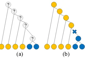
Figure 1: Phylogenetic comparative methods. Each node denotes a language with its state, or the value of its feature, indicated by color. (a) The task set-tings. A tree and the states of the leaf nodes are ob-served. The states of the internal nodes are latent variables to be inferred. (b) A result of inference. The cross sign on the branch indicates a change of the state.
field of evolutionary biology (Dediu,2010; Green-hill et al., 2010; Dunn et al., 2011;Maurits and Griffiths, 2014; Greenhill et al., 2017). As illus-trated in Figure 1, the key idea is that if a phy-logenetic tree is given, we can infer the ances-tral states with varying degrees of confidence, and by extension, can induce diachronic universals of change. To perform statistical inference, we as-sume that each feature evolves along the branches of the tree according to a continuous-time Markov chain (CTMC) model, which is controlled by a transition rate matrix(TRM). Once TRMs are es-timated, we can gain insights from them, for ex-ample, by simulating language evolution (Maurits and Griffiths,2014).
One problem in previous studies is that they do not adequately model a characteristic of typolog-ical features that has been central to linguistic ty-pology, that is, the fact that these features are not independent but depend on each other (Greenberg,
1 1 0 … 0 2 1 … 3
features x𝑙𝑙,∗
parameters z𝑙𝑙,∗
Step 1.Map each language into the latent representation
Step 2.Infer a set of transition rate matrices using phylo. trees (also infer the states and dates of the internal nodes)
1 1 0 … 0 1 0 0 … 0 0 0 1 … 1 1 0 0 … 0
0 0 1 … 1
0 1 1 … 1 1 1 1 … 0 1 1 1 … 0
0
tim
e
bef
ore
pres
en
t
Q𝑘𝑘= 0.0002∗ 0.0003∗
transition rate matrices (TRMs)
Step 3.Simulate language evolution using TRMs
1 1 0 … 0
parameters z𝑙𝑙,∗
time 𝑡𝑡 Q𝑘𝑘=0.0002∗ 0.0003∗
1 0 0 … 1
parameters z𝑙𝑙′,∗
1 1 … 2
features x𝑙𝑙′,∗ infer
[image:2.595.104.271.272.351.2]gen.
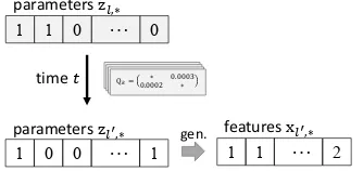
Figure 2: Overview of our framework. Observed and latent variables are marked in gray and white, respectively.
(NRel) (VO → NRel, in shorthand), and a re-lated universal, RelN → OV, also holds (Dryer,
2011). Despite the long-standing interest in inter-feature dependencies, most statistical models as-sume independence between features (Daum´e III,
2009;Dediu, 2010;Greenhill et al., 2010, 2017;
Murawaki,2016;Murawaki and Yamauchi,2018). A rare exception is Dunn et al. (2011), who ex-tended Greenberg’s idea by applying a phyloge-netic model of correlated evolution (Pagel and Meade, 2006). However, the model adopted by
Dunn et al.(2011) can only handle the dependency between a pair of binary features. Typological fea-tures have two or more possible values in general, and more importantly, the dependencies between features are not limited to a pair (Itoh and Ueda,
2004). For example, the order of relative clauses has connections to the order of adjective and noun (AdjNorNAdj), in addition to the order of object and verb, as two universals,RelN → AdjN and NAdj → NRel, are known to hold well (Dryer,
2011).
In this paper, we propose latent representation-based analysis of diachronic typology. Figure 2
shows an overview of our framework.
Follow-ingMurawaki(2017), we assume that a sequence of discrete surface features that represents a lan-guage is generated from a sequence of binary la-tent variables called parameters (Step 1). Pa-rameters are, by assumption, independent of each other and switching one parameter entails multi-ple changes of surface features in general. Thus, by performing phylogenetic inference on the la-tent space, we can handle the dependencies of all available features in an implicit manner (Step 2). The latent parameter representation can be pro-jected back to the surface feature representation when needed for analysis. LikeMaurits and Grif-fiths(2014), we run simulation experiments to in-terpret the estimated model parameters (Step 3).
What we propose is a general framework with which we can analyze any discrete feature, but as a proof-of-concept demonstration, we follow Mau-rits and Griffiths(2014) in focusing on the order of subject, object and verb (hereafter simply referred to as basic word order or BWO).1 In the dataset we use, the BWO feature has 7 possible values, 6 logically possible orders plus the special value No dominant order (Dryer, 2013b), mean-ing that it cannot be analyzed directly withDunn et al.’s model. We show that languages sharing the same word order are not a coherent group but exhibit varying degrees of diachronic stability de-pending on other features.
2 Related Work
2.1 Statistical Diachronic Typology
The building block of statistical phylogenetic models2 is a time-tree, which places nodes on an axis of time. In their standard applications to language (Gray and Atkinson, 2003; Bouckaert et al.,2012), time-trees are inferred from cognate
1
We chose the BWO feature because it is appealing to a wider audience. We are aware that Matthew S. Dryer, who provided language data for the BWO feature, favors binary classifications (OVvs. VOandSVvs. VS) over the six-way classification (Dryer,1997,2013a). He argues that the binary classifications are more fundamental than the six-way clas-sification, but our latent representation-based analysis does not require feature values to be primitive in nature because it reorganizes feature values into various latent parameters.
2
Statistical phylogenetic models can be either distance-based and character-distance-based. Character-distance-based models are clas-sified into parsimony-based and likelihood-based. In this pa-per, we focus on likelihood-based Bayesian models for their ability to date internal nodes. However, it is worth noting that attempts to overcome the limitations of the tree model mostly rely on non-likelihood-based models (Nakhleh et al.,2005;
Dep. # of language families Tree sources Dating Abs.
Dediu(2010) single 1 experts yes no
Greenhill et al.(2010) single 1 cognates no yes
Maurits and Griffiths(2014) single 1or7combined other no yes
Dunn et al.(2011) bin. pair 1 cognates no yes
[image:3.595.75.522.62.146.2]Ours all 309incl.154isolates experts yes yes
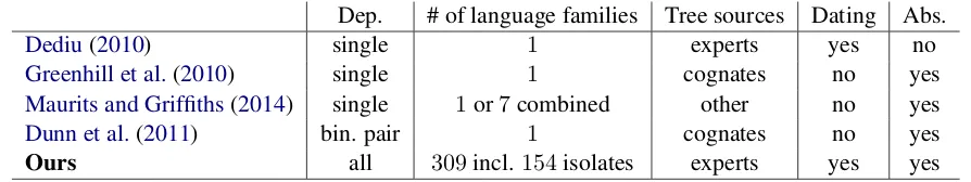
Table 1: A comparison of time-tree-based approaches to diachronic typology. (1) Feature dependencies modeled: independent (single), a pair of binary features (bin. pair) or all dependencies considered (all). (2) The number of language families (i.e., trees) used for each run of phylogenetic inference. (3) The sources of the trees used in inference: tree topologies established by historical linguists (experts), time-trees reconstructed by phylogenetic models using cognate data (cognates), or time-time-trees obtained by distance-based clustering based on geographical coordinates or others (other). (4) Whether the dates of internal nodes are inferred (yes) or given a priori (no). (5) Whether absolute dates are obtained. If no, only dates relative to the root node are inferred.
data (Dyen et al., 1992; Greenhill et al., 2008).3 However, if a tree is given a priori, phylogenetic models can also be used to estimate the parameters of a TRM, which controls how languages change their feature values over time. This is how typo-logical features are analyzed in previous studies.
Dediu(2010) aggregated TRMs taken from var-ious families to measure the stability of features.
Greenhill et al.(2010) compared typological data with cognate data in terms of stability. Maurits and Griffiths(2014) focused on the BWO feature and analyzed how it had changed in the past and was likely to change in the future. Dunn et al.
(2011) estimated TRMs for pairs of binary fea-tures and found that perceived correlated evolution was mostly lineage-specific rather than universal.
Taking a closer look at these studies, we can see that they vary as to how to prepare trees, as sum-marized in Table 1. Leaf nodes are assumed to be at the present datet = 0, but how can we as-sign backward dates tto internal nodes? A pop-ular approach (Greenhill et al.,2010;Dunn et al.,
2011) is to construct a time-tree with absolute (cal-endar) dates, using binary-coded lexical cognate data, and then to fit each trait of interest indepen-dently on the time-tree.4
However, cognate data are available only for a handful of language families such as Indo-European, Austronesian and Niger-Congo (or its mammoth Bantu branch). Moreover, phylogenetic
3 See Pereltsvaig and Lewis (2015) for a criticism of
computational approaches to historical linguistics andChang
et al.(2015) for an elegant solution to a set of problems
com-monly found in inferred time-trees.
4To be precise, a set of tree
samplesgiven by MCMC
sam-pling is usually employed to account for uncertainty.
inference was performed separately one after the other. This marks a sharp contrast with the long tradition of testing against a worldwide sample. In fact, it is suggested that sample diversity and ag-gregate time depth are not large enough to draw meaningful conclusions (Croft et al.,2011;Levy and Daum´e III,2011).
For this reason, we take another approach, which was employed by Dediu (2010). He used language families established by historical lin-guists. Because such tree topologies are not as-sociated with dates, he inferred the dates of in-ternal nodes together with the states of inin-ternal nodes and TRMs. This was possible because he jointly fitted a sequence of traits, instead of fitting each trait independently. If multiple traits are com-bined, they provide considerable information on a branch length, or the time elapsing from a parent to a child, because the elapsed time is roughly in-versely proportional to the similarity between the two nodes.5
Our approach differs from Dediu’s mainly in two points. First, whereas Dediu (2010) per-formed posterior inference separately for each lan-guage family, we tie a single set of TRMs to all available language families. Second,Dediu(2010) only inferred relative dates because he did not perform calibration (Drummond and Bouckaert,
2015). In order to assign calendar dates to nodes, we use multiple calibration points (the clock in Figure2indicates a calibration point). As is
com-5
monly done in the cognate-based reconstruction of a time-tree (Bouckaert et al.,2012), we set the Gaussian, Gaussian mixture, log-normal and uni-form distributions as priors on the dates of the cor-responding internal nodes.
2.2 Latent Representations of Languages
While previous studies analyzed the evolution of a single categorical feature (Dediu,2010;Greenhill et al.,2010;Maurits and Griffiths,2014) or a pair of binary features (Dunn et al.,2011), we capture the dependencies of all available features by map-ping each language to a sequence of independent latent variables. To our knowledge, Murawaki
(2015) was the first to introduce latent representa-tions to typological features. Pointing out several critical problems, however, Murawaki(2017) su-perseded the earlier model. The present study is built on top of a slightly modified version of the Bayesian model presented byMurawaki(2017).
Like the present study, Murawaki (2015) per-formed phylogenetic inference on the latent space. However, since this model lacks the notion of time, it does not have descriptive power beyond clustering. Borrowing statistical models from the field of evolutionary biology, we perform time-aware inference.
3 Proposed Method
3.1 Latent Representations of Languages
Central to our framework of diachronic analysis are the latent representations of languages ( Mu-rawaki, 2017). Each language l is represented as a sequence of N discrete features xl,∗ = (xl,1,· · ·, xl,N) ∈ NN0 . xl,n can take a binary
value (xl,n ∈ {0,1}) or categorical value (xl,n ∈
{1,2,· · · , Fn}, where Fn is the number of
dis-tinct values). We assume thatxl,∗is stochastically
generated from its latent representation, zl,∗ = (zl,1,· · ·, zl,K) ∈ {0,1}K, where K is the
num-ber of binary parameters, which is given a priori. Dependencies between surface features are cap-tured by weight matrixW ∈ RK×M. M will be
described below. In the generative story, we first calculate feature score vector θ˜l,∗ = (zTl,∗W)T ∈
RM. We then obtain model parameter vector
θl,∗ ∈(0,1)M by normalizingθ˜l,∗for each feature
type n. We use the sigmoid function for binary features,
θl,f(n,1) =
1
1 + exp(−θ˜l,f(n,1))
, (1)
and the softmax function for categorical features,
θl,f(n,i) =
exp(˜θl,f(n,i))
PFn
i0=1exp(˜θl,f(n,i0))
. (2)
Note that while a binary feature corresponds to one model parameter, categorical feature n is tied to Fn model parameters. We use
func-tion f(n, i) ∈ {1,· · · , m,· · ·, M} to map fea-ture n to the corresponding model parameter in-dex. Finally, we draw a binary feature from
Bernoulli(θl,f(n,1)), and a categorical feature fromCategorical(θl,f(n,1),· · · , θl,f(n,Fn)).
To gain an insight into how W captures inter-feature dependencies, suppose that for parameter k, a certain group of languages takezl,k = 1. If
two categorical feature values(n1, i1)and(n2, i2) have large positive weights (i.e., wk,f(n1,i1) > 0
andwk,f(n2,i2) > 0), then the pair must often co-occur in these languages because W raises both θl,f(n1,i1) and θl,f(n2,i2). Likewise, the fact that
two feature values do not co-occur can be encoded as a positive weight for one value and a negative weight for the other.
The remaining question is howzl,kis generated.
We drawz∗,k = (z1,k,· · ·, zL,k) from an
autolo-gistic model (Besag, 1974) that incorporates the observation that phylogenetically or areally close languages tend to take the same value.
To complete the generative story, letXandZbe the matrices of languages in the surface and latent representations, respectively, and letAbe a set of latent variables controllingKautologistic models. The joint distribution is defined as
P(A, Z, W, X)=P(A)P(Z|A)P(W)P(X|Z, W),
where hyperparameters are omitted for brevity. For prior probabilitiesP(A)andP(W), please re-fer toMurawaki(2017).
Even if less than 30% of the items of X are present, this model has been demonstrated to re-cover missing values reasonably well. Also, when plotted on a world map, some parameters appear to retain phylogenetic and areal signals observed for surface features, indicating that they are not mere statistical artifacts (Murawaki,2017).
3.2 Transition Rate Matrices (TRMs)
model (Drummond and Bouckaert, 2015). The CTMC is a continuous extension to the more fa-miliar discrete-time Markov chain. It is is con-trolled by a TRMQk. If the number of states
(pos-sible values) is2, thenQkis a2×2matrix:
Qk=
−αk αk
βk −βk
.
We set Gamma priors onαk, βk>0.
Qkcan be used to calculate thetransition
prob-ability, or the probability of language l taking valuebfor parameterkconditioned onl’s parent π(l)andt, the time span between the two:
P(zl,k=b|zπ(l),k =a, t) = exp(tQk)a,b. (3)
The matrix exponential exp(tQk) can be solved
analytically ifQkis a2×2matrix:
exp(tQk)=
βk+αke−(αk+βk)t αk+βk
αk−αke−(αk+βk)t αk+βk βk−βke−(αk+βk)t
αk+βk
αk+βke−(αk+βk)t αk+βk
!
.
Astapproaches to infinity, we obtain the station-ary probability( βk
αk+βk, αk αk+βk)
T. We can see that
αk andβk control both the speed of change (the
larger the higher) and the stationary distribution. A root node has no parent by definition. We draw the state of a root node from the stationary distribution. Thus, language isolates do have im-pact on posterior inference of TRMs.
3.3 Posterior Inference of Time-trees
To estimate TRMs, we need to specify the gen-erative model of time-trees and an inference al-gorithm. In the generative story, each tree topol-ogy is drawn from some uniform distribution. The dates of its nodes are determined next. If the node in question is not a calibration point, its date is drawn from some uniform distribution, subject to the ancestral ordering constraint: a node must be older than its descendants. If the node is a calibra-tion point, its date is drawn from the correspond-ing prior distribution.6 TRM parameters,αk and
βk, are generated from Gamma priors. For the root
node, the value of parameterkis drawn from the corresponding stationary distribution. The states of the non-root nodes are generated using Eq. (3). Given tree topologies, the states of the leaf nodes and calibration points, we need to infer
6This model is slightly leaky because some priors (e.g.,
Gaussian) assign non-zero probabilities to illogical time-trees that violate the ancestral ordering constraint.
(1) the dates of the internal nodes, (2) the states of the internal nodes, and (3) TRM parameters,αk
andβk, for each latent parameter k. Gibbs
sam-pling updates of these variables are as follows:
Update dates We update the dates of the inter-nal nodes one by one. The time span in which the target node can move is bound by its parent (if there is) and its eldest child. We use slice sam-pling (Neal,2003) to update the date. In addition, we use a Metropolis-Hastings operator that multi-plies the dates of all the internal nodes of a tree by a rate drawn from a log-normal distribution.
Update states For each parameterk, we block-sample a whole given tree. Specifically, we implement a Bayesian version of Felsenstein’s tree-pruning algorithm, which is akin to the for-ward filtering-backfor-ward sampling algorithm for Bayesian hidden Markov models.
Updateαkandβk We jointly sampleαkandβk
for eachk. Since both the transition and station-ary probabilities can be obtained analytically for binary traits, we use Hamiltonian Monte Carlo to exploit gradient information (Neal,2011).
3.4 Three-Step Analysis
Now we are ready to elaborate on the proposed framework of diachronic analysis (Figure2).
Step 1 We map each language, represented as a sequence of N discrete surface features, to a se-quence ofK binary latent parameters. Let feature matrixXbe decomposed into observed and miss-ing portions,Xobs andXmis, respectively. Given Xobs, we use Gibbs sampling to inferA, param-eter matrixZ, weight matrixW, and Xmis (
Mu-rawaki,2017).7
In the present study, we setK = 100. We run
5independent MCMC chains. For each chain, we start with 1,000 burn-in iterations. We then ob-tain10 samples with an interval of10 iterations. Note that after burn-in iterations, we fix W and only sampleA,Z, andXmisto avoid the identifi-ability problems (e.g., label-switching). For each item ofZ andXmis, we output the most frequent value among the10samples. We do this to reduce uncertainty.
7We employ a slightly modified Metropolis-Hastings
Step 2 We fit a set ofK TRMs on family trees around the world. Formally, what are observed are tree topologies, the states of the leaf nodes (i.e., sequences of latent parameters), and multiple cali-bration points. Given these, we infer TRM param-eters, αk andβk, for each latent parameter k, as
well as the dates and states of the internal nodes. We, again, use Gibbs sampling as explained in Section3.3.
We collect10samples with an interval of10 it-erations after1,000burn-in iterations. We do this for each of the5samples obtained in Step 1. As a result, we obtain50samples in total.
Step 3 We analyze the TRMs by simulating lan-guage evolution. Given the latent representation of languagel, we stochastically generate its descen-dant l0 after some time span t. Specifically, we drawzl0,kaccording to the transition probability of Eq. (3) for each parameterk. Using weight matrix W, we then project the latent representation zl0,∗ back to the surface representationxl0,∗. To be pre-cise, we use model parameter vectorθl0,∗, instead of xl0,∗, for further analysis. For each of the 50 samples obtained in Step 2, we simulate the evolu-tion of a given language100times (5,000samples in total).
4 Experiments
4.1 Data and Preprocessing
The database of typological features we used is the online edition8of theWorld Atlas of Language Structures(WALS) (Haspelmath et al.,2005). We preprocessed the database as was done in Mu-rawaki(2017), with different thresholds. As a re-sult, we obtained a language–feature matrix con-sisting of L = 2,607 languages and N = 152
features. Only19.98% of items in the matrix were present. We manually classified features into bi-nary and categorical ones. The number of model parameters,M, was760.
We used Glottolog 3.2 (Hammarstr¨om et al.,
2018) as the source of family trees. Glottolog has three advantages over Ethnologue (Lewis et al.,
2014), another commonly-used catalog of the world’s languages. (1) Glottolog makes explicit that it adopts a genealogical classification, rather than hierarchical clusterings of modern languages. (2) It reflects more recent research. (3) Map-ping between Glottolog and WALS is easy
be-8http://wals.info/
cause WALS provides Glottolog’s language codes (glottocodes) when available.
After Step 1 of Section 3.4, we dropped lan-guages from WALS that could not be mapped to Glottolog. As a result,2,557languages remained. We subdivided a Glottolog node if multiple lan-guages from WALS shared the same glottocode. We removed leaf nodes that were not present in WALS and repeatedly dropped internal nodes that had only one child. We obtained 309 language families among which154had only one node (i.e., language isolates).
We collected 50 calibration points from sec-ondary literature (Holman et al.,2011;Bouckaert et al., 2012;Gray et al.,2009;Maurits and Grif-fiths, 2014;Grollemund et al.,2015). For exam-ple, we set a Gaussian prior with mean2,500BP (before present) and standard deviation500on the date of (Proto-)Hmong-Mien. See Table S.1 of the supplementary materials for details. Our calibra-tion points are by no means definitive or exhaus-tive but should be seen as a first step toward world-scale dating.
4.2 Case Study: Basic Word Order (BWO)
As a proof-of-concept demonstration of the pro-posed framework, we investigate the BWO fea-ture, or WALS’s Feature 81A (Dryer,2013b). The cross-linguistic variation of BWO attracts atten-tion not only from typologists but from psycholin-guists (seeMaurits and Griffiths(2014) for a brief review). Some claim that the fact thatSOV is the most frequent order indicates its optimality, pre-sumably in terms of functionality. Some others point to an apparent historical trend ofSOV chang-ing to SVO, but not vice versa (Gell-Mann and Ruhlen, 2011), which might imply (1) the func-tional superiority ofSVOoverSOVand (2) an even higher prevalence ofSOVin the past.SOV prefer-ences in emerging sign languages (Sandler et al.,
2005) and in elicited pantomime (Goldin-Meadow et al.,2008) are also reported.
Maurits and Griffiths(2014) fitted a6×6TRM9 on large language families. However, we sus-pect that singling out BWO is oversimplification. Given its profound effect on the whole grammati-cal system, a BWO change can hardly occur inde-pendently of other features. In fact,Mithun(1995) lists a variety of morphological factors that have
9The special value No dominant order was
SOV SVO VSO VOS OVS OSV ndo. SOV
SVO
VSO
VOS OVS
OSV
ndo. 0.1
[image:7.595.75.291.66.208.2]0.2 0.3 0.4 0.5 0.6 0.7 0.8
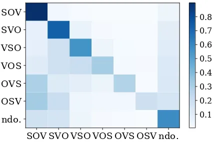
Figure 3: Transition probability of BWO. An item of the matrix(a, b) indicates how probable a lan-guage with word order awill take word order b after 2,000years. Note that this covers the sce-nario in which the language switches to another word ordercbefore changing tob.
diachronically reduced the rigidity of SOV order in Native American languages. Her analysis sug-gests that languages sharing the same word order might not be a monolithic group.
Here, we use latent representation-based anal-ysis to answer questions: how variable language sharing the same BWO are with respect to di-achronic stability, and what kind of features are correlated with BWO stability?
4.3 Variability of Diachronic Stability
Among the 2,557 modern languages, we chose
1,357languages for which the BWO feature was present. We simulated evolution witht = 2,000, as described in Section 3.4. Let n be the index of the BWO feature. For the 5,000 samples of each simulated languagel0, we averaged the BWO probability vectors,θl0,f(n,1),· · · , θl0,f(n,F
n).
Before going into inter-language variability, let us take a look at the overall trend. We took the average of the BWO probability vectors for each word order. The result is shown in Figure3. Our findings largely agree with those of Maurits and Griffiths (2014): (1) SOV is the most diachroni-cally stable word order, which is followed bySVO, (2) SOV prefers changing to SVO over VSO (al-though hardly visually recognizable), and (3)VSO is more likely to change toSVOthan toSOV, just to name a few.
Next, the variability is visualized in Figure 4. We can see that languages sharing the same word order differ considerably in terms of diachronic
SOV
SVO VSO
VOS OVS
OSV
0.0 0.2 0.4 0.6 0.8 1.0
[image:7.595.311.526.66.215.2]No dominant order
Figure 4: Variability in the probability of keep-ing the same word order. For word order i, the x-axis indicates the average ofθl0,f(n,i), the proba-bility of taking word orderiafter2,000years. The y-axis indicates the relative frequency of the cor-responding probability among the languages with word orderi. Kernel density estimation is used for smoothing. The pulse in each box shows the corre-sponding probability estimated by directly fitting the7×7TRM of the surface feature.
stability. For comparison, we fitted the7×7TRM of the BWO feature on the samples of time-trees obtained in Step 2 of Section 3.4. For SOV and SVO, the probabilities based on the surface fea-ture pointed to the modal probabilities based on the latent representations. This is somewhat sur-prising because we anticipated that the combina-tion of the stochastic surface-to-latent and latent-to-surface mappings would amplify uncertainty of estimation.
The two least common word orders, OVS (0.8%) and OSV (0.3%) exhibited huge gaps be-tween the two types of probabilities. The proba-bilities based on the surface feature were consis-tently larger (i.e., more stable). Surface feature-based estimation had no other way to explain the presence of these uncommon word orders than slowing down the convergence to the stationary distribution (otherwise they go extinct). Maurits and Griffiths(2014) also reported some counter-intuitive results regardingOVS andOSV. By con-trast, latent parameter-based estimation appears to have explained the low frequencies partly with the stochasticity of observation associated with the latent-to-surface mapping.
ana-Weight Explanatory variable (feature: value)
0.01527 59A Possessive Classification: More than five classes
0.01297 90A Order of Relative Clause and Noun: Relative clause-Noun
0.01138 85A Order of Adposition and Noun Phrase: Postpositions
0.00998 94A Order of Adverbial Subordinator and Clause: Final subordinator word
0.00889 51A Position of Case Affixes: Case suffixes
−0.02507 93A Position of Interrogative Phrases in Content Questions: Initial interrogative phrase
−0.02576 26A Prefixing vs. Suffixing in Inflectional Morphology: Weakly prefixing
−0.02738 143E Preverbal Negative Morphemes: NegV
−0.03169 85A Order of Adposition and Noun Phrase: Inpositions
[image:8.595.307.525.61.262.2]−0.08360 85A Order of Adposition and Noun Phrase: No dominant order
Table 2: Regression analysis of variability forSOV.
10among94variables are shown.
lyze their complex dependencies. The approach we adopt in the present study is to let a sim-pler model explain the model’s complex behav-ior. Specifically, we used linear regression with L1 regularization (i.e., lasso). The hyperparameter was tuned using 3-fold cross-validation. For each word orderi, the target variable was the average of θl0,f(n,i) while explanatory variables were the current surface features, xl,1,· · · , xl,N. For
bet-ter inbet-terpretability, we excluded from explanatory variables surface features that trivially depended on the BWO feature (Takamura et al.,2016). Note that missing values were imputed in Step 1 of Sec-tion3.4.
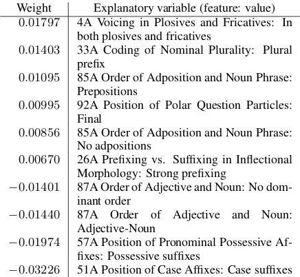
Tables 2 and 3 show the results of regres-sion analysis forSOVandSVOlanguages, respec-tively. As expected, feature values typically asso-ciated with the specified word order had positive weights while negative weights indicate inconsis-tency. A stable SOVlanguage may use prenomi-nal relative clauses, postpositions and/or case suf-fixes. The trend was less clear forSVOlanguages, but those characterized by heavy use of prefixes were stable too. Interestingly, Feature 85A (Or-der of Adposition and Noun Phrase) had two posi-tively weighted values:PrepositionsandNo adpositions. We speculate that SVO order is suitable for analytic languages that rely heav-ily on word ordering to encode syntactic structure (e.g., English and languages of Mainland South-east Asia) but is not necessarily so for languages with rich morphological devices for marking
syn-Weight Explanatory variable (feature: value)
0.01797 4A Voicing in Plosives and Fricatives: In both plosives and fricatives
0.01403 33A Coding of Nominal Plurality: Plural prefix
0.01095 85A Order of Adposition and Noun Phrase: Prepositions
0.00995 92A Position of Polar Question Particles: Final
0.00856 85A Order of Adposition and Noun Phrase: No adpositions
0.00670 26A Prefixing vs. Suffixing in Inflectional Morphology: Strong prefixing
−0.01401 87A Order of Adjective and Noun: No dom-inant order
−0.01440 87A Order of Adjective and Noun: Adjective-Noun
−0.01974 57A Position of Pronominal Possessive Af-fixes: Possessive suffixes
−0.03226 51A Position of Case Affixes: Case suffixes
Table 3: Regression analysis of variability forSVO.
10among52variables are shown.
Prob. Language Family Aff.
0.854 Fyam Atlantic-Congo WS
0.828 Younuo Bunu Hmong-Mien LA
0.825 Czech Indo-European WS
0.825 Tetum Austronesian LA
0.824 Stieng Austroasiatic LA
0.824 Alune Austronesian EQ
0.822 Berom Atlantic-Congo SP
0.822 Paulohi Austronesian EQ
0.821 South-Central Kikongo Atlantic-Congo SP
0.820 Abun (isolate) LA
Table 4: Some of the most stable SVO languages with the values of the affixation feature (Dryer,
2013c). The first column indicates the probabil-ities of keeping the SVO order after 2,000years. Names of languages and language families are taken from Glottolog. The values of the affixation feature areEQ(Equal prefixing and suffixing),LA (Little affixation), SP(Strong prefixing), and WS (Weakly suffixing).
tactic structure so that word ordering can relatively freely convey information structure.
4.4 Language-Specific Analysis
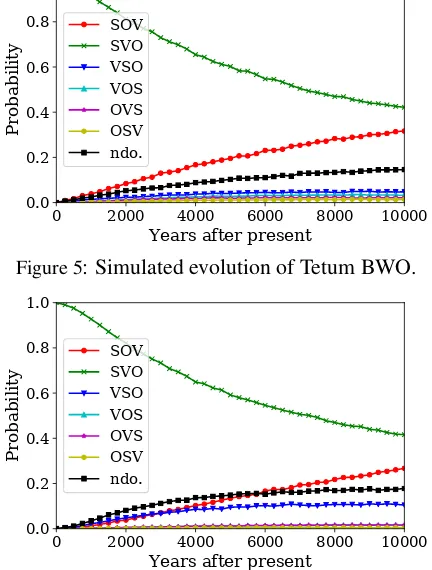
In Section4.3, we suggested that stableSVO lan-guages do not form a coherent group but can be grouped into at least two clusters. This can be con-firmed in Table4, where most of the most stable SVO languages exhibit either (1) little affixation or (2) strong prefixation. To analyze these lan-guages in detail, we performed language-specific simulations. We chose Tetum and South-Central Kikongo as the examples of analytic and strongly prefixing languages, respectively.
[image:8.595.308.525.304.418.2]0 2000 4000 6000 8000 10000
Years after present
0.0 0.2 0.4 0.6 0.8 1.0
Probability
[image:9.595.307.528.61.184.2]SOV SVO VSO VOS OVS OSV ndo.
Figure 5: Simulated evolution of Tetum BWO.
0 2000 4000 6000 8000 10000
Years after present
0.0 0.2 0.4 0.6 0.8 1.0
Probability
[image:9.595.75.287.67.219.2]SOV SVO VSO VOS OVS OSV ndo.
Figure 6: Simulated evolution of South-Central Kikongo BWO.
Tetum as a function of time. For each time t, we performed simulation 500 times for each of the50samples and took the average of the BWO probability vectors,θl0,f(n,1),· · · , θl0,f(n,F
n).
Ac-cording to our analysis, Tetum will remain SVO with a probability of 81.1% at t = 2,000. SVO was followed bySOV(8.4%) andNo dominant order(5.3%).
What will the Austronesian language of East Timor look like in the future, if it switches toSOV? To answer this question, we performed regression analysis again witht = 2,000. For each word or-deri, the target variable wasθl0,f(n,i)of each sam-ple of simulated languagel0 whereas explanatory variables were the items of the probability vec-torθl0,∗. In other words, we aimed at finding out features that were characteristic of the specified word order. As before, we removed surface tures with trivial dependencies on the BWO fea-ture (Takamura et al.,2016) as well as the BWO feature itself.
Table 5 shows the result of regression analy-sis. If the relatively analytic language switches to SOV, Tetum will be characterized by a holis-tic reconfiguration. It is likely to develop suf-fixes and to replace prepositions with
postposi-Weight Explanatory variable (feature: value)
0.1256 85A Order of Adposition and Noun Phrase: Postpositions
0.1086 16A Weight Factors in Weight-Sensitive Stress Systems: Coda consonant
0.0687 69A Position of Aspect Affixes: Tense-aspect suffixes
0.0552 35A Plurality in Independent Personal Pro-nouns: Number-indifferent pronouns
0.0518 2A Vowel Quality Inventories: Large (7-14)
0.0506 122A Relativization on Subjects: Non-reduction
Table 5: Regression analysis of the Tetum chang-ing toSOVorder. Top6out of262variables.
Weight Explanatory variable (feature: value)
0.1048 15A Weight-Sensitive Stress: Left-oriented: One of the first three
0.0940 85A Order of Adposition and Noun Phrase: Postpositions
0.0821 16A Weight Factors in Weight-Sensitive Stress Systems: Coda consonant
0.0715 7A Glottalized Consonants: Ejectives, implo-sives, and glottalized resonants
0.0661 100A Alignment of Verbal Person Marking: Accusative
0.0636 64A Nominal and Verbal Conjunction: Both expressed by juxtaposition
Table 6: Regression analysis of the South-Central Kikongo changing toSOVorder. Top6out of408
variables.
tions. South-Central Kikongo is analyzed in the same manner, as shown in Figure 6and Table 6. The Bantu language of Africa is markedly differ-ent from Tetum as it is characterized by a higher tendency to switch toNo dominant order.
5 Conclusion
In this paper, we presented a new framework of latent representation-based analysis of diachronic typology, which enables us to investigate corre-lated evolution of multiple surface features in an exploratory manner. We focused on the order of subject, object and verb as a proof-of-concept demonstration, but investigating other features would be fruitful too. We analyzed the estimated model parameters with simulation experiments. In the future, we would like to investigate the inferred trees in detail.10 The source code is publicly
avail-able at https://github.com/murawaki/
lattyp.
Acknowledgments
This work was partly supported by JSPS KAK-ENHI Grant Number 18K18104.
10A preliminary analysis is presented in Section S.2 of the
[image:9.595.73.289.81.366.2]References
Julian Besag. 1974. Spatial interaction and the statisti-cal analysis of lattice systems. Journal of the Royal Statistical Society. Series B (Methodological), pages 192–236.
Balthasar Bickel. 2013. Distributional biases in lan-guage families. In David A. Peterson and Alan Tim-berlake, editors,Language Typology and Historical Contingency, pages 415–444. John Benjamins.
Remco Bouckaert, Philippe Lemey, Michael Dunn, Simon J. Greenhill, Alexander V. Alekseyenko, Alexei J. Drummond, Russell D. Gray, Marc A. Suchard, and Quentin D. Atkinson. 2012. Mapping the origins and expansion of the Indo-European lan-guage family. Science, 337(6097):957–960.
Will Chang, Chundra Cathcart, David Hall, and An-drew Garrett. 2015. Ancestry-constrained phyloge-netic analysis supports the Indo-European steppe hy-pothesis.Language, 91(1):194–244.
William Croft, Tanmoy Bhattacharya, Dave Klein-schmidt, D. Eric Smith, and T. Florian Jaeger. 2011. Greenbergian universals, diachrony, and statistical analyses. Linguistic Typology, 15(2):433–453.
Hal Daum´e III. 2009. Non-parametric Bayesian areal linguistics. In Proceedings of Human Language Technologies: The 2009 Annual Conference of the North American Chapter of the Association for Computational Linguistics, pages 593–601.
Hal Daum´e III and Lyle Campbell. 2007. A Bayesian model for discovering typological implications. In
Proceedings of the 45th Annual Meeting of the Asso-ciation of Computational Linguistics, pages 65–72.
Dan Dediu. 2010. A Bayesian phylogenetic approach to estimating the stability of linguistic features and the genetic biasing of tone. Proceedings of the Royal Society of London B: Biological Sciences, 278(1704):474–479.
Alexei J. Drummond and Remco R. Bouckaert. 2015.
Bayesian Evolutionary Analysis with BEAST. Cam-bridge University Press.
Matthew S. Dryer. 1997. On the six-way word order ty-pology. Studies in Language. International Journal sponsored by the Foundation “Foundations of Lan-guage”, 21(1):69–103.
Matthew S. Dryer. 2011. The evidence for word order correlations: a response to Dunn, Greenhill, Levin-son and Gray’s paper in Nature. Linguistic Typol-ogy, 15:335–380.
Matthew S. Dryer. 2013a. On the six-way word order typology, again. Studies in Language. International Journal sponsored by the Foundation “Foundations of Language”, 37(2):267–301.
Matthew S. Dryer. 2013b. Order of subject, object and verb. In Matthew S. Dryer and Martin Haspelmath, editors,The World Atlas of Language Structures On-line. Max Planck Institute for Evolutionary Anthro-pology.
Matthew S. Dryer. 2013c. Prefixing vs. suffixing in inflectional morphology. In Matthew S. Dryer and Martin Haspelmath, editors,The World Atlas of Lan-guage Structures Online. Max Planck Institute for Evolutionary Anthropology.
Michael Dunn, Simon J. Greenhill, Stephen C. Levin-son, and Russell D. Gray. 2011. Evolved structure of language shows lineage-specific trends in word-order universals. Nature, 473(7345):79–82.
Isidore Dyen, Joseph B. Kruskal, and Paul Black. 1992. An Indoeuropean classification: A lexicostatistical experiment. Transactions of the American Philo-sophical Society, 82(5):1–132.
Joseph Felsenstein. 1981. Evolutionary trees from DNA sequences: A maximum likelihood approach.
Journal of Molecular Evolution, 17(6):368–376.
Murray Gell-Mann and Merritt Ruhlen. 2011. The ori-gin and evolution of word order. Proceedings of the National Academy of Sciences, 108(42):17290– 17295.
Susan Goldin-Meadow, Wing Chee So, Aslı ¨Ozy¨urek, and Carolyn Mylander. 2008. The natural order of events: How speakers of different languages repre-sent events nonverbally. Proceedings of the National Academy of Sciences, 105(27):9163–9168.
Russell D. Gray and Quentin D. Atkinson. 2003. Language-tree divergence times support the Ana-tolian theory of Indo-European origin. Nature, 426(6965):435–439.
Russell D. Gray, Alexei J. Drummond, and Simon J. Greenhill. 2009. Language phylogenies reveal ex-pansion pulses and pauses in Pacific settlement. sci-ence, 323(5913):479–483.
Joseph H. Greenberg. 1963. Some universals of gram-mar with particular reference to the order of mean-ingful elements. In Joseph H. Greenberg, editor,
Universals of Language, pages 73–113. MIT Press.
Joseph H. Greenberg. 1978. Diachrony, synchrony and language universals. In Joseph H. Greenberg, Charles A. Ferguson, and Edith A. Moravesik, ed-itors, Universals of Human Language, volume 1. Stanford University Press.
Simon J. Greenhill, Robert Blust, and Russell D. Gray. 2008. The Austronesian basic vocabulary database: From bioinformatics to lexomics. Evolutionary Bioinformatics, 4:271–283.
Simon J. Greenhill, Chieh-Hsi Wu, Xia Hua, Michael Dunn, Stephen C. Levinson, and Russell D. Gray. 2017. Evolutionary dynamics of language systems.
Proceedings of the National Academy of Sciences, 114(42):E8822–E8829.
Rebecca Grollemund, Simon Branford, Koen Bostoen, Andrew Meade, Chris Venditti, and Mark Pagel. 2015. Bantu expansion shows that habitat alters the route and pace of human dispersals. Proceedings of the National Academy of Sciences, 112(43):13296– 13301.
Harald Hammarstr¨om, Robert Forkel, Martin Haspel-math, and Sebastian Bank, editors. 2018. Glottolog 3.2. Max Planck Institute for the Science of Human History.
Martin Haspelmath, Matthew Dryer, David Gil, and Bernard Comrie, editors. 2005. The World Atlas of Language Structures. Oxford University Press.
Eric W. Holman, Cecil H. Brown, Søren Wich-mann, Andr´e M¨uller, Viveka Velupillai, Harald Hammarstr¨om, Sebastian Sauppe, Hagen Jung, Dik Bakker, Pamela Brown, Oleg Belyaev, Matthias Ur-ban, Robert Mailhammer, Johann-Mattis List, and Dmitry Egorov. 2011. Automated dating of the world’s language families based on lexical similar-ity.Current Anthropology, 52(6):841–875.
Yoshiaki Itoh and Sumie Ueda. 2004. The Ising model for changes in word ordering rules in natu-ral languages. Physica D: Nonlinear Phenomena, 198(3):333–339.
Roger Levy and Hal Daum´e III. 2011. Computational methods are invaluable for typology, but the mod-els must match the questions. Linguistic Typology, 15:393–399.
M. Paul Lewis, Gary F. Simons, and Charles D. Fen-nig, editors. 2014. Ethnologue: Languages of the World, 17th Edition. SIL International. Online ver-sion: http://www.ethnologue.com.
Elena Maslova. 2000. A dynamic approach to the ver-ification of distributional universals. Linguistic Ty-pology, 4(3):307–333.
Luke Maurits and Thomas L. Griffiths. 2014. Trac-ing the roots of syntax with Bayesian phylogenetics.
Proceedings of the National Academy of Sciences, 111(37):13576–13581.
Marianne Mithun. 1995. Morphological and prosodic forces shaping word order. In Pamela A. Downing and Michael Noonan, editors, Word Order in Dis-course, pages 387–423. John Benjamins Publishing.
Yugo Murawaki. 2015. Continuous space representa-tions of linguistic typology and their application to phylogenetic inference. InProceedings of the 2015 Conference of the North American Chapter of the Association for Computational Linguistics: Human Language Technologies, pages 324–334.
Yugo Murawaki. 2016. Statistical modeling of creole genesis. InProceedings of the 2016 Conference of the North American Chapter of the Association for Computational Linguistics: Human Language Tech-nologies, pages 1329–1339.
Yugo Murawaki. 2017. Diachrony-aware induction of binary latent representations from typological fea-tures. In Proceedings of the Eighth International Joint Conference on Natural Language Processing (Volume 1: Long Papers), pages 451–461. Asian Federation of Natural Language Processing.
Yugo Murawaki and Kenji Yamauchi. 2018. A statisti-cal model for the joint inference of vertistatisti-cal stability and horizontal diffusibility of typological features.
Journal of Language Evolution, 3(1):13–25.
Luay Nakhleh, Don Ringe, and Tandy Warnow. 2005. Perfect phylogenetic networks: A new methodology for reconstructing the evolutionary history of natural languages. Language, pages 382–420.
Radford M. Neal. 2003. Slice sampling. Annals of Statistics, 31(3):705–767.
Radford M. Neal. 2011. MCMC using Hamilto-nian dynamics. In Steve Brooks, Andrew Gelman, Galin L. Jones, and Xiao-Li Meng, editors, Hand-book of Markov Chain Monte Carlo, pages 113–162. CRC Press.
Shijulal Nelson-Sathi, Johann-Mattis List, Hans Geisler, Heiner Fangerau, Russell D. Gray, William Martin, and Tal Dagan. 2010. Networks uncover hidden lexical borrowing in Indo-European lan-guage evolution. Proceedings of the Royal Society B: Biological Sciences.
Johanna Nichols. 1992. Linguistic Diversity in Space and Time. University of Chicago Press.
Mark Pagel and Andrew Meade. 2006. Bayesian anal-ysis of correlated evolution of discrete characters by reversible-jump Markov chain Monte Carlo. The American Naturalist, 167(6):808–825.
Asya Pereltsvaig and Martin W. Lewis. 2015. The Indo-European Controversy: Facts and Fallacies in Historical Linguistics. Cambridge University Press.