SCFG Decoding Without Binarization

SCFG Decoding Without Binarization

Mark Hopkins and Greg Langmead SDL Language Weaver, Inc. 6060 Center Drive, Suite 150

Los Angeles, CA 90045

{mhopkins,glangmead}@languageweaver.com

Abstract

Conventional wisdom dictates that syn-chronous context-free grammars (SCFGs) must be converted to Chomsky Normal Form (CNF) to ensure cubic time decoding. For ar-bitrary SCFGs, this is typically accomplished via the synchronous binarization technique of (Zhang et al., 2006). A drawback to this ap-proach is that it inflates the constant factors as-sociated with decoding, and thus the practical running time. (DeNero et al., 2009) tackle this problem by defining a superset of CNF called Lexical Normal Form (LNF), which also sup-ports cubic time decoding under certain im-plicit assumptions. In this paper, we make these assumptions explicit, and in doing so, show that LNF can be further expanded to a broader class of grammars (called “scope-3”) that also supports cubic-time decoding. By simply pruning non-scope-3 rules from a GHKM-extracted grammar, we obtain better translation performance than synchronous bi-narization.

1 Introduction

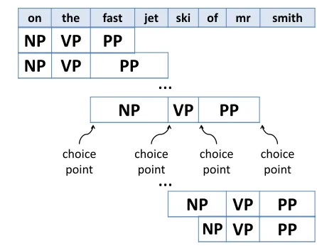
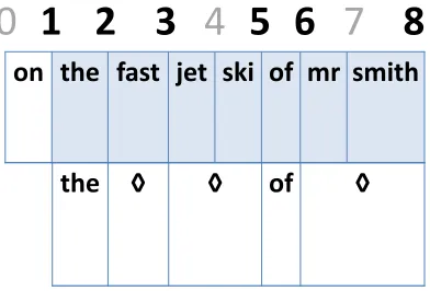
At the heart of bottom-up chart parsing (Younger, 1967) is the following combinatorial problem. We have a context-free grammar (CFG) rule (for in-stance, S → NP VP PP) and an input sentence of length n (for instance, “on the fast jet ski of mr smith”). During chart parsing, we need to apply the rule to all relevant subspans of the input sentence. See Figure 1. For this particular rule, there are n+1₄

application contexts, i.e. ways to choose the

sub-spans. Since the asymptotic running time of chart parsing is at least linear in this quantity, it will take

on the fast jet ski of mr smith

NP VP

PP

NP VP

PP

NP

VP

PP

NP

_VP

_PP

NP

VP

PP

choice point

choice point

choice point

choice point

…

…

Figure 1: A demonstration of application contexts. There are n+1₄

application contexts for the CFG rule “S→NP VP PP”, wherenis the length of the input sentence.

at leastO( n+1₄

) = O(n4) time if we include this rule in our grammar.

Fortunately, we can take advantage of the fact that any CFG has an equivalent representation in Chom-sky Normal Form (CNF). In CNF, all rules have the form X→ Y Z or X→ x, where x is a termi-nal and X, Y, Z are nontermitermi-nals. If a rule has the form X→ Y Z, then there are only n+1₃ applica-tion contexts, thus the running time of chart parsing isO( n+1₃ ) = O(n3)when applied to CNF gram-mars.

A disadvantage to CNF conversion is that it in-creases both the overall number of rules and the overall number of nonterminals. This inflation of the “grammar constant” does not affect the asymp-totic runtime, but can have a significant impact on the performance in practice. For this reason,

the NPB of NNP

on the fast jet ski of mr smith

the NPB of NNP

on the fast jet ski of mr smith

the JJ NPB of NNP

the JJ NPB of NNP

the JJ NPB of NNP

the JJ NPB of NNP

choice point

choice point choice point

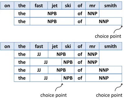
Figure 2: A demonstration of application contexts for rules with lexical anchors. There are O(n) application contexts for CFG rule “S → the NPB of NNP”, and O(n2_{) application contexts for CFG rule “S → the JJ}

NPB of NNP”, if we assume that the input sentence has lengthnand contains no repeated words.

ero et al., 2009) provide a relaxation of CNF called Lexical Normal Form (LNF). LNF is a superclass of CNF that also allows rules whose right-hand sides have no consecutive nonterminals. The intuition is that the terminals provide anchors that limit the ap-plicability of a given rule. For instance, consider the rule NP→the NPB of NNP. See Figure 2. Because the terminals constrain our choices, there are only two different application contexts. The implicit as-sumption is that input sentences will not repeat the same word more than a small constant number of times. If we make the explicit assumption that all words of an input sentence are unique, then there are O(n2) application contexts for a “no consecu-tive nonterminals” rule. Thus under this assumption, the running time of chart parsing is stillO(n3)when applied to LNF grammars.

But once we make this assumption explicit, it be-comes clear that we can go even further than LNF and still maintain the cubic bound on the runtime. Consider the rule NP → the JJ NPB of NNP. This rule is not LNF, but there are still only O(n2) ap-plication contexts, due to the anchoring effect of the terminals. In general, for a rule of the form X→ γ, there are at mostO(np)application contexts, where pis the number of consecutive nonterminal pairs in

the string X·γ·X (where X is an arbitrary nontermi-nal). We refer topas thescopeof a rule. Thus chart parsing runs in timeO(nscope(G)), wherescope(G) is the maximum scope of any of the rules in CFGG. Specifically, any scope-3 grammar can be decoded in cubic time.

Like (DeNero et al., 2009), the target of our in-terest is synchronous context-free grammar (SCFG) decoding with rules extracted using the GHKM al-gorithm (Galley et al., 2004). In practice, it turns out that only a small percentage of the lexical rules in our system have scope greater than 3. By simply re-moving these rules from the grammar, we can main-tain the cubic running time of chart parsing without any kind of binarization. This has three advantages. First, we do not inflate the grammar constant. Sec-ond, unlike (DeNero et al., 2009), we maintain the

synchronousproperty of the grammar, and thus can

integrate language model scoring into chart parsing. Finally, a system without binarized rules is consid-erably simpler to build and maintain. We show that this approach gives us better practical performance than a mature system that binarizes using the tech-nique of (Zhang et al., 2006).

2 Preliminaries

Assume we have a global vocabulary of symbols, containing the reservedsubstitution symbol♦. De-fine asentence as a sequence of symbols. We will typically use space-delimited quotations to represent example sentences, e.g. “the fast jet ski” rather than

hthe,fast,jet,skii. We will use the dot operator to represent the concatenation of sentences, e.g. “the fast”·“jet ski” = “the fast jet ski”.

Define the rank of a sentence as the count of its ♦ symbols. We will use the no-tation SUB(s, s1, ..., sk) to denote the

substitu-tion of k sentences s1, ..., sk into a k-rank

sen-tence s. For instance, if s = “the ♦ ♦ of

♦”, then SUB(s,“fast”,“jet ski”,“mr smith”) = “the fast jet ski of mr smith”.

To refer to a subsentence, define aspanas a pair [a, b]of nonnegative integers such that a < b. For a sentences=hs1, s2, ..., sniand a span[a, b]such

NP -> the JJ NN of NNP

PP -> on NP

JJ -> fast NN -> jet ski NNP -> mr smith

NP -> < the JJ₁NN₂of NNP₃, le NN₂JJ₁de NNP₃>

PP -> < on NP

, sur NP

>

JJ -> < fast, vite > NN -> < jet ski, jet ski > NNP -> < mr smith, m smith >

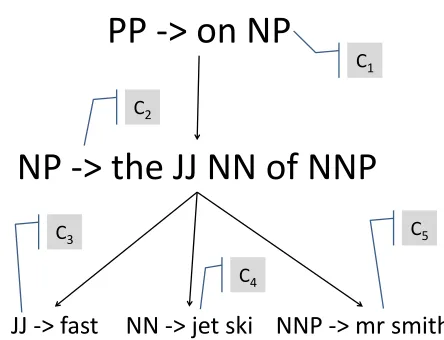
Figure 3: An example CFG derivation (above) and an ex-ample SCFG derivation (below). Both derive the sen-tence SUB(“on _♦”, SUB( “the _{♦ ♦} of _♦”, “fast”, “jet ski”, “mr smith”) ) = “on the fast jet ski of mr smith”. The SCFG derivation simultaneously derives the auxil-iary sentence “sur le jet ski vite de m smith”.

3 Minimum Derivation Cost

Chart parsing solves a problem which we will re-fer to as Minimum Derivation Cost. Because we want our results to be applicable to both CFG decod-ing and SCFG decoddecod-ing with an integrated language model, we will provide a somewhat more abstract formulation of chart parsing than usual.

In Figure 3, we show an example of a CFG deriva-tion. A derivation is a tree of CFG rules, constructed so that thepreconditions(the RHS nonterminals) of any rule match thepostconditions (the LHS nonter-minal) of its child rules. The purpose of a derivation is to derive a sentence, which is obtained through recursive substitution. In the example, we substitute “fast”, “jet ski”, and “mr smith” into the lexical pat-tern“the♦ ♦of♦” to obtain “the fast jet ski of mr smith”. Then we substitute this result into the lexi-cal pattern “on♦” to obtain “on the fast jet ski of mr smith”.

The cost of a derivation is simply the sum of the base costs of its rules. Thus the cost of the CFG derivation in Figure 3 isC1+C2+C3+C4+C5,

whereC1is the base cost of rule “PP→on NP”, etc.

Notice that this cost can be distributed locally to the nodes of the derivation (Figure 4).

An SCFG derivation is similar to a CFG

deriva-NP -> the JJ NN of Nderiva-NP

PP -> on NP

JJ -> fast

NN -> jet ski NNP -> mr smith

C3

C4

C5

C2

C1

Figure 4: The cost of the CFG derivation in Figure 3 is C1 +C2+C3+C4 +C5, where C1 is the base cost

of rule “PP→on NP”, etc. Notice that this cost can be distributed locally to the nodes of the derivation.

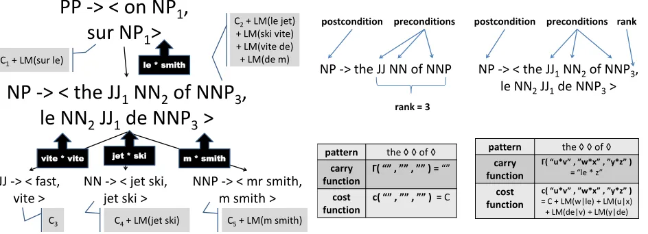
tion, except that it simultaneously derives two sen-tences. For instance, the SCFG derivation in Fig-ure 3 derives the sentence pairh“on the fast jet ski of mr smith”, “sur le jet ski vite de m smith”i. In machine translation, often we want the cost of the SCFG derivation to include a language model cost for this second sentence. For example, the cost of the SCFG derivation in Figure 3 might beC1+C2+C3+ C4+C5+LM(sur le)+LM(le jet)+LM(jet ski)+ LM(ski de) +LM(de m) +LM(m smith), where LMis the negative log of a 2-gram language model. This new cost function can also be distributed lo-cally to the nodes of the derivation, as shown in Fig-ure 5. However, in order to perform the local com-putations, we need to pass information (in this case, the LM boundary words) up the tree. We refer to this extra information ascarries. Formally, define a

carryas a sentence of rank 0.

In order to provide a chart parsing formulation that applies to both CFG decoding and SCFG de-coding with an integrated language model, we need abstract definitions of rule and derivation that cap-ture the above concepts of pattern, postcondition,

preconditions,cost, andcarries.

3.1 Rules

NP -> < the JJ

NN

of NNP

,

le NN

JJ

de NNP

>

PP -> < on NP

,

sur NP

>

JJ -> < fast, vite >

NN -> < jet ski, jet ski >

NNP -> < mr smith, m smith > m * smith

C5+ LM(m smith)

C4+ LM(jet ski)

C3

vite * vite jet * ski le * smith

C2+ LM(le jet)

+ LM(ski vite) + LM(vite de) + LM(de m) C1+ LM(sur le)

Figure 5: The cost of the SCFG derivation in Figure 3 (with an integrated language model score) can also be dis-tributed to the nodes of the derivation, but to perform the local computations, information must be passed up the tree. We refer to this extra information as acarry.

sentence called thepattern1,X is a symbol called thepostcondition,πis ak-length sentence called the

preconditions,Γis a function (called thecarry func-tion) that maps a k-length list of carries to a carry, and c is a function (called the cost function) that maps ak-length list of carries to a real number. Fig-ure 6 shows a CFG and an SCFG rule, deconstructed according to this definition.2 Note that the CFG rule has trivial cost and carry functions that map every-thing to a constant. We refer to such rules assimple. We will usepost(r) to refer to the postcondition of ruler, andpre(r, i)to refer to theithprecondition of ruler.

Finally, define agrammaras a finite set of rules. A grammar issimpleif all its rules are simple.

3.2 Derivations

For a grammarR, definederiv(R)as the smallest set that contains every tuplehr, δ1, ..., δkisatisfying the

following conditions:

1

For simplicity, we also impose the condition that “♦” is not a valid pattern. This is tantamount to disallowing unary rules.

2_{One possible point of confusion is why the pattern of the} SCFG rule refers only to the primary sentence, and not the aux-iliary sentence. To reconstruct the auxaux-iliary sentence from an SCFG derivation in practice, one would need to augment the abstract definition of rule with an auxiliary pattern. However this is not required for our theoretical results.

NP -> < the JJ1NN2of NNP3,

le NN2JJ1de NNP3>

postcondition preconditions rank

pattern the ◊ ◊ of ◊

carry function

Γ( “u*v” , ”w*x” , ”y*z” ) = “le * z”

cost function

c( “u*v” , ”w*x” , ”y*z” ) = C + LM(w|le) + LM(u|x) + LM(de|v) + LM(y|de)

NP -> the JJ NN of NNP

postcondition preconditions

pattern the ◊ ◊ of ◊

carry function

Γ( “” , ”” , ”” ) = “”

cost function

c( “” , ”” , ”” ) = C

rank = 3

Figure 6: Deconstruction of a CFG rule (left) and SCFG rule (right) according to the definition of rule in Sec-tion 3.1. The carry funcSec-tion of the SCFG rule computes boundary words for a 2-gram language model. In the cost functions,Cis a real number and LM returns the negative log of a language model query.

• r∈Ris ak-rank rule

• δi∈deriv(R)for all1≤i≤k

• pre(r, i) =post(ri)for all1≤i≤k, whereri

is the first element of tupleδi.

AnR–derivationis an element ofderiv(R). Con-sider a derivation δ = hr, δ1, ..., δki, where rule

r = hk, s∗, X, π,Γ, ci. Define the following prop-erties:

post(δ) =post(r)

sent(δ) =SUB(s∗,sent(δ1), ...,sent(δk))

carry(δ) = Γ(carry(δ1), ...,carry(δk))

cost(δ) =c(carry(δ1), ...,carry(δk)) + k X

j=1

cost(δj)

In words, we say that derivation δ derives sen-tencesent(δ). If for some spanσof a particular sen-tences, it holds thatsent(δ) =sσ, then we will say

thatδis a derivationoverspanσ.

3.3 Problem Statement

on the fast jet ski of mr smith

the

◊

◊

of

◊

0

1 2 3

4

5 6

7

8

Figure 7: An application context for the pattern “the_{♦ ♦} of_♦” and the sentence “on the fast jet ski of mr smith”.

s, find the minimum cost of anyR–derivation that derivess. In other words, compute:

MinDCost(R, s), min

δ∈deriv(R)|sent(δ)=scost(δ)

4 Application Contexts

Chart parsing solves Minimum Derivation Cost via dynamic programming. It works by building deriva-tions over increasingly larger spans of the input sen-tences. Consider just one of these spansσ. How do we build a derivation over that span?

Recall that a derivation takes the form

hr, δ1, ..., δki. Given the rule r and its pattern

s∗, we need to choose the subderivations δi such

that SUB(s∗,sent(δ1), ...,sent(δk)) = sσ. To do

so, we must match the pattern to the span, so that we know which subspans we need to build the subderivations over. Figure 7 shows a matching of the pattern “the ♦ ♦ of♦” to span [1,8] of the sentence “on the fast jet ski of mr smith”. It tells us that we can build a derivation over span[1,8]by choosing this rule and subderivations over subspans [2,3],[3,5], and[6,8].

We refer to these matchings as application

con-texts. Formally, given two sentences s∗ and s

of respective lengths m and n, define an hs∗, si–

context as an monotonically increasing sequence

hx0, x1, ..., xmi of integers between 0 and n such

that for alli:

s∗_[i−1,i]6=♦implies thats∗_[i−1,i]=s[xi−1,xi]

The context shown in Figure 7 is h1,2,3,5,6,8i. Use cxt(s∗, s) to denote the set of all hs∗, si– contexts.

An hs∗, si–context x = hx0, x1, ..., xmi has the

following properties:

span(x;s∗, s) = [x0, xm]

subspans(x;s∗, s) =h[x0, x1], ...,[xm−1, xm]i

Moreover, define varspans(x;s∗, s) as the sub-sequence of subspans(x;s∗, s) including only [xi−1, xi] such that s∗_[i−1,i] = ♦. For the context

xshown in Figure 7:

span(x;s∗, s) = [1,8]

subspans(x;s∗, s) =h[1,2],[2,3],[3,5],[5,6],[6,8]i varspans(x;s∗, s) =h[2,3],[3,5],[6,8]i

An application context x ∈ cxt(s∗, s) tells us that we can build a derivation overspan(x)by choosing a rule with patterns∗ and subderivations over each span invarspans(x;s∗, s).

5 Chart Parsing Algorithm

We are now ready to describe the chart parsing al-gorithm. Consider a span σ of our input sentence sand assume that we have computed and stored all derivations over any subspan ofσ. A naive way to compute the minimum cost derivation over spanσis to consider every possible derivation:

1. Choose a ruler=hk, s∗, X, π,Γ, ci.

2. Choose an application context x ∈ cxt(s∗, s) such thatspan(x;s∗, s) =σ.

3. For each subspan σi ∈ varspans(x;s∗, s),

choose a subderivationδi such thatpost(δi) =

pre(r, i).

Chart parsing takes advantage of the above obser-vation to avoid building all possible deriobser-vations. In-stead it groups together derivations that share a com-mon subspan, postcondition, and carry, and records only the minimum cost for each equivalence class. It records this cost in an associative map referred to as thechart.

Specifically, assume that we have computed and stored the minimum cost of every derivation class

hσ0, X0, γ0i, where X0 is a postcondition, γ0 is a carry, andσ0 is a proper subspan of σ. Chart pars-ing computes the minimum cost of every derivation classhσ, X, γiby adapting the above naive method as follows:

1. Choose a ruler=hk, s∗, X, π,Γ, ci.

2. Choose an application context x ∈ cxt(s∗, s) such thatspan(x;s∗, s) =σ.

3. For each subspan σi ∈ varspans(x;s∗, s), choose a derivation classhσi, Xi, γiifrom the chartsuch thatXi =pre(r, i).

4. Update3 the cost of derivation class hσ,post(r),Γ(γ1, ..., γk)iwith:

c(γ1, ..., γk) + k X

i=1

chart[σi, Xi, γi]

where chart[σi, Xi, γi] refers to the stored cost of derivation classhσi, Xi, γii.

By iteratively applying the above method to all sub-spans of size 1, 2, etc., chart parsing provides an efficient solution for the Minimum Derivation Cost problem.

6 Runtime Analysis

At the heart of chart parsing is a single operation: the updating of a value in the chart. The running time is linear in the number of these chart updates. 4 _{The typical analysis counts the number of chart} updates per span. Here we provide an alternative

3

Here, updatemeans “replace the cost associated with the class if the new cost is lower.”

4

This assumes that you can linearly enumerate the relevant updates. One convenient way to do this is to frame the enumer-ation problem as a search space, e.g. (Hopkins and Langmead, 2009)

analysis that counts the number of chart updatesper rule. This provides us with a finer bound with prac-tical implications.

Letr be a rule with rankkand pattern s∗. Con-sider the chart updates involving rule r. There is (potentially) an update for every choice of (a) span, (b) application context, and (c) list of kderivation classes. If we let C be the set of possible carries, then this means there are at most|cxt(s∗, s)| · |C|k

updates involving ruler.5 If we are doing beam de-coding (i.e. after processing a span, the chart keeps only theB items of lowest cost), then there are at most|cxt(s∗, s)| ·Bkupdates.

We can simplify the above by providing an upper bound for |cxt(s∗, s)|. Define an ambiguity as the sentence “♦ ♦”, and definescope(s∗)as the number of ambiguities in the sentence “♦” ·s∗· “♦”. The following bound holds:

Lemma 1. Assume that a zero-rank sentencesdoes not contain the same symbol more than once. Then

|cxt(s∗, s)| ≤ |s|scope(s∗)_.

Proof. Supposes∗ andshave respective lengthsm

andn. Considerhx0, x1, ..., xmi ∈ cxt(s∗, s). Let

I be the set of integersibetween1andmsuch that s∗_i 6= ♦and letI+be the set of integers ibetween 0andm−1such thats∗_i+1 6= ♦. Ifi∈ I, then we know the value ofxi, namely it is the unique integer

j such thatsj = s∗i. Similarly, ifi ∈ I+, then the

value of xi must be the unique integer j such that

sj = s∗i+1. Thus the only nondetermined elements

of contextxiare those for whichi6∈I∪I+. Hence |cxt(s∗, s)| ≤ |s|{0,1,...,m}−I−I+

=|s|scope(s∗₎

.

Hence, under the assumption that the input sen-tencesdoes not contain the same symbol more than once, then there are at most|s|scope(s∗)_{· |C|}k _chart

updates involving a rule with patterns∗.

For a rule r with pattern s∗, define scope(r) =

scope(s∗). For a grammar R, define scope(R) = maxr∈Rscope(r)andrank(R) = maxr∈Rrank(r).

Given a grammar R and an input sentence s, the above lemma tells us that chart parsing makes

5

O(|s|scope(R) _{· |C|}rank(R)_{) chart updates. If we}

re-strict ourselves to beam search, than chart parsing makesO(|s|scope(R)_{)chart updates.}6

6.1 On the Uniqueness Assumption

In practice, it will not be true that each input sen-tence contains only unique symbols, but it is not too far removed from the practical reality of many use cases, for which relatively few symbols repeat them-selves in a given sentence. The above lemma can also be relaxed to assume only that there is a con-stant upper bound on the multiplicity of a symbol in the input sentence. This does not affect the O-bound on the number of chart updates, as long as we further assume a constant limit on the length of rule patterns.

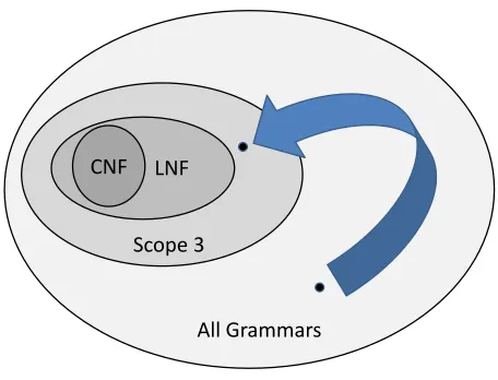
7 Scope Reduction

From this point of view, CNF binarization can be viewed as a specific example of scope reduction. Suppose we have a grammarRof scopep. See Fig-ure 8. If we can find a grammarRˆ of scopep < pˆ which is “similar” to grammarR, then we can de-code inO(npˆ)rather thanO(np)time.

We can frame the problem by assuming the fol-lowing parameters:

• a grammarR

• a desired scopep

• a loss function Λ that returns a (non-negative real-valued) score for any two grammarsRand

ˆ

R; ifΛ(R,Rˆ) = 0, then the grammars are con-sidered to be equivalent

Ascope reduction method with lossλfinds a

gram-mar Rˆ such thatscope( ˆR) ≤ p andΛ(R,Rˆ) = λ. A scope reduction method is losslesswhen its loss is 0.

In the following sections, we will use the loss function:

Λ(R,Rˆ) =|MinDCost(R, s)−MinDCost( ˆR, s)|

where s is a fixed input sentence. Observe that if Λ(R,Rˆ) = 0, then the solution to the Minimum

6_{Assumingrank(R)is bounded by a constant.}

CNF LNF

Scope 3

All Grammars

Figure 8: The “scope reduction” problem. Given a gram-mar of large scope, find a similar gramgram-mar of reduced scope.

Derivation Cost problem is the same for bothRand ˆ

R. 7

7.1 CNF Binarization

A rulerisCNFif its pattern is “♦ ♦” or “x”, where x is any non-substitution symbol. A grammar isCNF

if all of its rules are CNF. Note that the maximum scope of a CNF grammar is 3.

CNF binarization is a deterministic process that

maps a simple grammar to a CNF grammar. Since binarization takes subcubic time, we can decode with any grammar R in O(n3) time by converting R to CNF grammarRˆ, and then decoding withRˆ. This is a lossless scope reduction method.

What if grammar R is not simple? For SCFG grammars, (Zhang et al., 2006) provide a scope reduction method called synchronous binarization

with quantifiable loss. Synchronous binarization se-lects a “binarizable” subgrammarR0of grammarR, and then convertsR0 into a CNF grammarRˆ. The cost and carry functions of these new rules are con-structed such that the conversion from R0 to Rˆ is a lossless scope reduction. Thus the total loss of the method is|MinDCost(R, s)−MinDCost(R0, s)|. Fortunately, they find in practice thatR0usually con-tains the great majority of the rules ofR, thus they

a ◊ ◊

◊ ◊ a

a ◊ ◊ b

◊ a ◊ ◊

◊ ◊ a ◊

◊ ◊ ◊ a

a ◊ ◊ ◊

a b ◊ ◊

◊ ◊ a b

a ◊ ◊ b ◊

a ◊ ◊ b c

a b ◊ ◊ c

◊ a ◊ ◊ b

a ◊ b ◊ ◊

◊ ◊ a ◊ b

◊ ◊ ◊ a b

a ◊ ◊ ◊ b

a ◊ ◊ b ◊ c

a ◊ ◊ ◊ ◊ b

a ◊ ◊ b c ◊ ◊ d

a ◊ ◊ ◊ ◊ b ◊ c ◊ d

a ◊ ◊ b ◊ ◊ c ◊ ◊ d

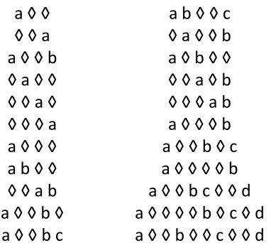
Figure 9: A selection of rule patterns that are scope≤3

but not LNF or CNF.

assert that this loss is negligable.

A drawback of their technique is that the resulting CNF grammar contains many more rules and post-conditions than the original grammar. These con-stant factors do not impact asymptotic performance, but do impact practical performance.

7.2 Lexical Normal Form

Concerned about this inflation of the grammar con-stant, (DeNero et al., 2009) consider a superset of CNF called Lexical Normal Form (LNF). A rule is

LNFif its pattern does not contain an ambiguity as a proper subsentence (recall that an ambiguity was defined to be the sentence “♦ ♦”). Like CNF, the maximum scope of an LNF grammar is 3. In the worst case, the pattern s∗ is “♦ ♦”, in which case there are three ambiguities in the sentence “♦”·s∗·

“♦”.

(DeNero et al., 2009) provide a lossless scope reduction method that maps a simple grammar to an LNF grammar, thus enabling cubic-time decod-ing. Their principal objective is to provide a scope reduction method for SCFG that introduces fewer postconditions than (Zhang et al., 2006). However unlike (Zhang et al., 2006), their method only ad-dresses simple grammars. Thus they cannot inte-grate LM scoring into their decoding, requiring them to rescore the decoder output with a variant of cube growing (Huang and Chiang, 2007).

0 0.1 0.2 0.3 0.4 0.5 0.6 0.7 0.8 0.9 1

0 1 2 3 4 5 6 7 8

%

o

f

ru

les

w

ith

sc

o

p

e

<=

P

P

AE Lexical CE Lexical AE Nonlexical CE Nonlexical

Figure 10: Breakdown of rules by scope (average per sen-tence in our test sets). In practice, most of the lexical rules applicable to a given sentence (95% for Arabic-English and 85% for Chinese-English) are scope 3 or less.

7.3 Scope Pruning

To exercise the power of the ideas presented in this paper, we experimented with a third (and very easy) scope reduction method calledscope pruning. If we consider the entire space of scope-3 grammars, we see that it contains a much richer set of rules than those permitted by CNF or LNF. See Figure 9 for examples. Scope pruning is a lossy scope reduc-tion method that simply takes an arbitrary grammar and prunes all rules with scope greater than 3. By not modifying any rules, we preserve their cost and carry functions (enabling integrated LM decoding), without increasing the grammar constant. The prac-tical question is: how many rules are we typically pruning from the original grammar?

Chinese-Arabic-English

Chinese-English

33 34 35 36 37 38 39 40

0 2000 4000 6000 8000

BL

EU

-4

Words per minute

27

28

29

30

31

32

33

34

35

36

37

0 2000 4000 6000 8000

BL

EU

-4

Words per minute

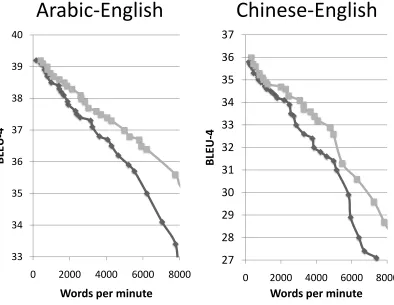
Figure 11: Speed-quality tradeoff curves comparing the baseline scope reduction method of synchronous binarization (dark gray diamonds) with scope-3 pruning (light gray squares).

English system, with rules extracted from 16 million words of parallel data from the mainland-news do-main of the LDC corpora, and with a 4-gram lan-guage model trained on monolingual English data from the AFP and Xinhua portions of the LDC Gi-gaword corpus. We evaluated this system’s perfor-mance on the NIST 2003 test corpus, which con-sists of 919 Chinese sentences, with four English reference translations. For both systems, we report BLEU scores (Papineni et al., 2002) on untokenized, recapitalized output.

In practice, how many rules have scope greater than 3? To answer this question, it is useful to dis-tinguish betweenlexicalrules (i.e. rules whose pat-terns contain at least one non-substitution symbol)

andnon-lexicalrules. Only a subset of lexical rules

are potentially applicable to a given input sentence. Figure 10 shows the scope profile of these applicable

rules (averaged over all sentences in our test sets). Most of the lexical rules applicable to a given sen-tence (95% for Arabic-English, 85% for Chinese-English) are scope 3 or less. 8 Note, however, that scope pruning also prunes a large percentage of non-lexical rules.

Figure 11 compares scope pruning with the base-line technique of synchronous binarization. To gen-erate these speed-quality tradeoff curves, we de-coded the test sets with 380 different beam settings. We then plotted the hull of these 380 points, by elim-inating any points that were dominated by another (i.e. had better speed and quality). We found that this simple approach to scope reduction produced a better speed-quality tradeoff than the much more complex synchronous binarization.9

8

For contrast, the corresponding numbers for LNF are 64% and 53%, respectively.

8 Conclusion

In this paper, we made the following contributions:

• We provided an abstract formulation of chart parsing that generalizes CFG decoding and SCFG decoding with an integrated LM.

• We framedscope reductionas a first-class ab-stract problem, and showed that CNF binariza-tion and LNF binarizabinariza-tion are two specific solu-tions to this problem, each with their respective advantages and disadvantages.

• We proposed a third scope reduction technique calledscope pruning, and we showed that it can outperform synchronous CNF binarization for particular use cases.

Moreover, this work gives formal expression to the extraction heuristics of hierarchical phrase-based translation (Chiang, 2007), whose directive not to extract SCFG rules with adjacent nonterminals can be viewed as a preemptive pruning of rules with scope greater than 2 (more specifically, the prun-ing of non-LNF lexical rules). In general, this work provides a framework in which different approaches

totractability-focusedgrammar construction can be

compared and discussed.

References

David Chiang. 2007. Hierarchical phrase-based transla-tion. Computational Linguistics, 33(2):201–228. John DeNero, Mohit Bansal, Adam Pauls, and Dan Klein.

2009. Efficient parsing for transducer grammars. In

Proceedings of the Human Language Technology Con-ference of the NAACL, Main ConCon-ference.

Michel Galley, Mark Hopkins, Kevin Knight, and Daniel Marcu. 2004. What’s in a translation rule? In Pro-ceedings of HLT/NAACL.

Mark Hopkins and Greg Langmead. 2009. Cube pruning as heuristic search. InProceedings of EMNLP. Liang Huang and David Chiang. 2007. Forest rescoring:

Faster decoding with integrated language models. In

Proceedings of ACL.

the lexical rules and synchronously binarized the non-lexical rules. This had a similar performance to scope-pruning all rules. The opposite approach of scope-pruning the lexical rules and synchronously binarizing the non-lexical rules had a similar performance to synchronous binarization.

Kishore Papineni, Salim Roukos, Todd Ward, and Wei-Jing Zhu. 2002. Bleu: a method for automatic eval-uation of machine translation. InProceedings of 40th Annual Meeting of the Association for Computational Linguistics, pages 311–318.

Daniel Younger. 1967. Recognition and parsing of context-free languages in time n3_{. Information and}

Control, 10(2):189–208.