Using Personal Traits For Brand Preference Prediction

Using Personal Traits For Brand Preference Prediction

Chao Yang1_{, Shimei Pan}2_{, Jalal Mahmud}3_{, Huahai Yang}4_{,andPadmini Srinivasan}1

1_{Computer Science, The University of Iowa, Iowa City, IA, USA}

{chao-yang, padmini-srinivasan}@uiowa.edu

2_{University of Maryland, Baltimore County, Baltimore, MD, USA}

[email protected]

3_{IBM Research Almaden, Almaden, CA, USA}

[email protected]

4_{Juji Inc, Saratoga, CA, USA}

[email protected]

Abstract

In this paper, we present a comprehensive study of the relationship between an indi-vidual’s personal traits and his/her brand preferences. In our analysis, we included a large number of character traits such as personality, personal values and individual needs. These trait features were obtained from both a psychometric survey and au-tomated social media analytics. We also included an extensive set of brand names from diverse product categories. From this analysis, we want to shed some light on (1) whether it is possible to use personal traits to infer an individual’s brand preferences (2) whether the trait features automatically inferred from social media are good prox-ies for the ground truth character traits in brand preference prediction.

1 Introduction

Brand preference analysis is an important topic in marketing. To induce a desired brand choice, a marketer must understand the main factors that in-fluence a consumer’s brand preferences. This task is not easy since many factors may play a role in determining one’s brand preferences such as a consumer’s individual characteristics and prefer-ences as well as the properties of a brand (e.g., its perceived quality). Among consumer related factors, demographics such as age, gender and in-come have been studied extensively in marketing research (Evans, 1959; Elliott, 1994; Lin, 2002). In this study, we focus on analyzing a set of con-sumer characteristics, which have received less attention but with these features, potentially we can build more precise and more accurate brand preference prediction models. Especially, we fo-cus on three types of personal traits: personality,

personal values, and individual needs. Personal-ityis a combination of characteristics or qualities that form an individual’s distinctive character; Per-sonal valuesreflect what are important to different individuals and what motivate them in their deci-sion making. Moreover, all people have certain

needsthat they want to satisfy. Thus, analyzing a comprehensive set of personal traits may help us understand the way we react to a particular brand. Previously, the relationship between personal traits and brand preference/purchase decisions has drawn limited interest in marketing research due to the difficulty in obtaining consumer traits on a large scale. Among these efforts, Westfall found that differences exist between the personalities of the owners of convertible cars and those of stan-dard & compact cars (Westfall, 1962). Similarly, the congruence of personal and brand personal-ity was suggested to be a predictor of consumers’ brand preferences (Jamal and Goode, 2001; Dik-cius et al., 2013). However, Shank & Lang-meyer found personal traits less useful in building a strategic marketing tool (Shank and Langmeyer, 1994).

Given limited and sometimes conflicting results in previous research, in this study, we want to sys-tematically investigate the relationship between a comprehensive set of personal traits and brand preferences. Specifically, we want to shed some light on (1) whether it is possible to use personal traits to predict consumer’s brand preferences? (2) whether it is feasible to use automatically inferred personal traits to build brand preference prediction systems that are scalable?

Our study offers several significant contribu-tions to the field of brand preference analysis:

1. It is the first study that includes a comprehen-sive set of personal traits in brand preference analysis. Our current investigation includes

personality(5 general categories and 30

facets), personal values (5 dimensions) and

individual needs (12 dimensions). In con-trast, previous work typically only included a small number of personal traits (e.g., just 5 personality traits in (Hirsh et al., 2012)).

2. It is the first study that uses personal traits obtained from both psychometric evaluation and social media analytics. The traits scores derived from psychometric tests are more ac-curate, which allow us to focus on the re-lationship between personal traits and brand preferences without the distractions from the mistakes introduced by an automated trait in-ference system. However, since psychomet-ric tests require users to answer a large num-ber of survey questions, without sufficient in-centives, it is difficult to perform psychomet-ric evaluation for a large number of people. In contrast, automatically derived trait fea-tures based on social media analytics require no user effort, and can be applied to millions of social media users.

3. Our study involves diverse brand categories such as luxury car brands, retail brands, fast food brands, and household product brands (e.g., shampoo brands). With this data, we can investigate whether the relationship be-tween personal traits and brand preferences varies across multiple product categories.

Since the current study focuses on a compre-hensive set of consumer characteristics and pref-erences which does not include many important brand properties such as perceived quality, risk, price and market presence, the main goal of our in-vestigation is not to build a highly accurate brand preference prediction system. Instead, we want to first establish the feasibility of using derived trait features in building large-scale brand preference prediction systems. In the following, we first sum-marize some prior work, then describe the details of our experiments.

2 Related Work

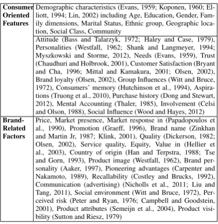
Predicting brand preference is a hard problem. A large number of factors may influence customers’ choices. Table 1 summarizes the factors that have been explored in previous research. Due to the scope, so far, there isn’t any prior investigation that is capable of incorporating all the factors in

a single model. Our study is one of the most com-prehensive analyses so far. We not only investi-gate the influence of a large number of personal traits but also combine them with other known consumer-related features such as demographics and personal interests. We however have not in-cluded any brand-related properties such as per-ceived quality, risk and market presence because we do not have access to these data.

Consumer Oriented Features

Demographic characteristics (Evans, 1959; Koponen, 1960; El-liott, 1994; Lin, 2002) including Age, Education, Gender, Fam-ily dimensions, Marital Status, Ethnic group, Geographic loca-tion, Social Class, Community

Attitude (Bass and Talarzyk, 1972; Haley and Case, 1979), Personalities (Westfall, 1962; Shank and Langmeyer, 1994; Myszkowski and Storme, 2012), Needs (Evans, 1959), Trust (Chaudhuri and Holbrook, 2001), Customer Satisfaction (Bryant and Cha, 1996; Mittal and Kamakura, 2001; Olsen, 2002), Brand loyalty (Olsen, 2002), Group Influences (Witt and Bruce, 1972), Consumers’ memory (Hutchinson et al., 1994), Aspira-tions (Truong et al., 2010), Purchase history (Dong and Stewart, 2012), Mental Accounting (Thaler, 1985), Involvement (Celsi and Olson, 1988), Social Influence (Wood and Hayes, 2012)

Brand-Related Factors

Price, Market presence, Market response in (Papadopoulos et al., 1990), Promotion (Graeff, 1996), Brand name (Zinkhan and Martin Jr, 1987; Klink, 2001), Quality (Dickerson, 1982; Olsen, 2002), Service quality, Equity, Value in (Hellier et al., 2003), Country of origin (Han and Terpstra, 1988; Tse and Gorn, 1993), Product image (Westfall, 1962), Brand per-sonality (Aaker, 1997), Pioneering advantages (Carpenter and Nakamoto, 1989), Recallability (Costley and Brucks, 1992), Communication (advertising) (Nicholls et al., 2011; Liu and Tang, 2011), Social environment (Witt and Bruce, 1972), Per-ceived risk (Peter and Ryan, 1976; Campbell and Goodstein, 2001), Product attributes (Semeijn et al., 2004), Product visi-bility (Sutton and Riesz, 1979)

Table 1: Features explored in previous studies

ex-plicitly express his opinion towards BMW (e.g. Driving BMW is exciting!). In contrast, with our system, if we know that he likes to seek excite-ment (exciteexcite-ment, a needs dimension) and enjoys luxury products (Hedonism, a values dimension), we can guess he may like BMW although he has never explicitly mentioned BMW in his social me-dia posts before. This difference is important since among the millions of products on social media, only a small number of products have been explic-itly rated/mentioned by a particular user.

In summary, brand preferences may be influ-enced by many consumer and brand-related fac-tors. Previous research has not paid sufficient at-tention to the influence of personal traits. In ad-dition, most previous studies used psychometric surveys which are impractical in mass marketing since it is unlikely that a large number of cus-tomers would take the time to answer lengthy sur-vey questions. In this study, we focus on inves-tigating the feasibility of using automatically in-ferred personal traits in large-scale brand prefer-ence prediction. Next, we describe the dataset we collected to support this study.

3 Data Collection

To investigate how personal traits are related to an individual’s brand preferences, we collected two datasets. In the first dataset, in addition to brand preferences, we also used standard psychometric tests to obtain clean and accurate personal trait measures. With this dataset, we can build and evaluate brand preference prediction models that use accurate personal traits. In contrast, the second dataset is used to build and evaluate brand prefer-ence prediction models that use trait features auto-matically inferred from social media. By compar-ing the models built from both datasets, we can answer questions such as: (1) whether personal traits are useful in predicting brand preferences (2) whether the traits automatically inferred from so-cial media are useful in predicting brand prefer-ences.

To collect these datasets, we designed two Ama-zon Mechanical Turk (MTurk) 1 _{tasks. All the}

MTurk participants are from the US since people outside the US may be unfamiliar with some of the brands. In the following, we describe the details of each MTurk task.

1_{http://mturk.com/}

Category Brand

Beverage (2) Coca-Cola, Pepsi Luxury Car (3) BMW, Cadillac, Lexus

Fast Food (4) Chipotle, McDonald’s, Panera Bread (PB) , Subway Retail (4) Kohl’s, Macy’s, Nordstrom, Target

Shampoo (4) Head & Shoulders (HS), Herbal Essences (HE),_{Pantene, Suave} Smart Phone (5) HTC, iPhone, Samsung, SONY, Nokia

Table 2: Selected brand categories and brands

3.1 Task 1: PTBP Survey

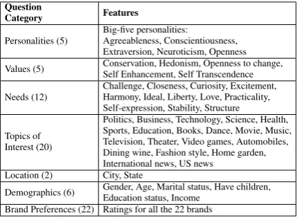
To collect the first dataset, we conducted a Per-sonal Traits & Brand Preferences (PTBP) survey. Our trait survey includes five parts designed to measure three types of personal traits: personal-ity, valuesandneedsplus demographics and per-sonal interests. Specifically, since the Big-Five model of personality is the most popular model of personality traits among personality psycholo-gists, we adopted a standard survey for Big 5 per-sonality. Here to limit the time MTurkers need to spend on the survey, instead of the full 300-item personality test, we used the shorter 50-item IPIP survey (Goldberg, 1993) which will score a user along 5 general personality dimensions: open-ness, conscientiousopen-ness, extraversion, agreeable-ness and neuroticism. However, with the shorter survey, we can not obtain the scores for 30 ad-ditional personality facets. Similarly, we used the standard 21-item PVQ survey to obtain the

tions. The validation questions are pairs of ques-tions that are paraphrases of each other. If the an-swers to a pair of validation questions are signif-icantly different, the user data are excluded from our analysis. Our final dataset has 1,017 valid re-sponses. Table 2 lists all the brands used in our study. All the measures used in our PTBP survey are listed in Table 3.

Question

Category Features

Personalities (5) Big-five personalities:Agreeableness, Conscientiousness, Extraversion, Neuroticism, Openness Values (5) Conservation, Hedonism, Openness to change,_{Self Enhancement, Self Transcendence}

Needs (12) Challenge, Closeness, Curiosity, Excitement,Harmony, Ideal, Liberty, Love, Practicality, Self-expression, Stability, Structure

Topics of Interest (20)

Politics, Business, Technology, Science, Health, Sports, Education, Books, Dance, Movie, Music, Television, Theater, Video games, Automobiles, Dining wine, Fashion style, Home garden, International news, US news

Location (2) City, State

Demographics (6) Gender, Age, Marital status, Have children,_{Education status, Income} Brand Preferences (22) Ratings for all the 22 brands

Table 3: PTBP Survey Feature Summary

3.2 Task 2: TAE Survey

The data collected in the Text Analytics Evalu-ation (TAE) survey are used to study the corre-lation between the trait features inferred from a person’s social media posts (e.g., tweets) and his brand preferences. Before the TAE survey, the participants were first asked to verify whether they had a Twitter account, if so, provide us their Twit-ter IDs. The users also agreed that we could access their tweets after the survey. Since our automated trait inference system relies on linguistic cues de-rived from a person’s Twitter posts, to ensure we can have a stable and reliable reading of one’s personal traits from his tweets, only active Twit-ter users with over 50 tweets (excluding retweets) can participate this survey. Since the majority of MTurkers are not active Twitter users, to increase the size of our data, in addition to MTurk, we also directly invited random Twitter users to participate in our TAE survey.

In addition to Twitter IDs, we also asked par-ticipants to provide their preferences for the same 22 brands as those used in the PTBP survey. Simi-larly, to filter out data by people who do not follow instructions, we also added two validation ques-tions. In total, in the TAE survey, we have col-lected data from 659 participants, out of which 608 are valid. (550 valid ones are from MTurk,

and 109 are from direct Twitter invitation).

3.3 Data Preparation

To obtain the trait scores for each user based on his answers in the PTBP survey, we first computed the raw trait scores based on the original survey guide-lines. Since different surveys used different scales, we normalized the trait scores by using their rank percentile (e.g., top 1%, top 5%). As a result, all the normalized personal trait scores are between 0 and 1.

Moreover, for each of the 20 topics of interest, we created a binary variable, indicating whether a participant is interested in a specific topic. In addition, each demographics feature such as age, education, income, was first mapped to an integer and then normalized into a number between 0 and 1.

To derive the trait scores for a user in the TAE survey, we crawled all the tweets in his Twitter account. Since personal traits are inferred from the text authored by a user, we discarded all the retweets. Due to the restrictions of the Twit-ter API, we can only crawl a maximum of 3,200 tweets for each user2_.

Recent research in psycholinguistics has shown it is possible to automatically infer personal traits from one’s linguistic footprints such as tweets and blogs (Yarkoni, 2010; Chen et al., 2014; Yang and Li, 2013). Here, we used a similar ap-proach. Specifically, given input text authored by a user (e.g., tweets), our system computed the word counts of different psychologically-meaningful word categories defined in the Linguistic Inquiry and Word Count (LIWC) dictionary (Pennebaker et al., 2001). The LIWC counts were then used to build prediction models to correlate one’s word usage with his ground truth personal traits ob-tained via a prior psychometric survey. Then the built models were used to automatically infer a user’s personal traits. Based on a preliminary eval-uation with 250 participants, more than 80 per-cent of them, scores for traits that were inferred for all three models correlated significantly with survey-based scores (p<0.05 and correlation coef-ficient between 0.05 and 0.8). Specifically, scores that were derived by our system correlated with survey-based scores for 80.8% of participants’Big Five scores (p<0.05 and correlation coefficients between 0.05 and 0.75), for 86.6% of participants’

Needs scores (p<0.05 and correlation coefficient between 0.05 and 0.8), and for 98.21% of partic-ipants’Valuesscores (p<0.05 and correlation co-efficients between 0.05 and 0.55). Moreover, the participants also rated on a five-point scale how well each derived characteristic matched their per-ceptions of themselves, and their ratings suggest that the inferred characteristics largely matched their self-perceptions. Specifically, means of all ratings were above 3 (“somewhat”) out of 5 (“per-fect”): 3.4 (with a std. of 1.14) forBig Five, 3.39 (with a std. of 1.34) forNeeds, and 3.13 (with a std. of 1.17) forValues.

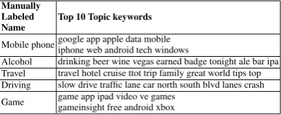
In addition to personal traits, we also included topics of interest in the TAE dataset. They were automatically inferred from tweets using Latent Dirichlet Allocation (LDA) (Blei et al., 2003). Since we need a large Twitter dataset to mine a list of general topics of interest, our current tweet col-lection is not sufficient. Therefore, we use a sep-arate and much larger Twitter dataset from 10,000 randomly selected Twitter users. For each user, we crawled his tweets and then aggregated them into a big document, one for each Twitter user. As a re-sult, we have 10,000 documents in our dataset. We then built an LDA topic model using this dataset. From the LDA inference results, we can infer a user’s topics of interest. Basically, for a given user u, LDA outputs a per user topic distributionΘu,

which is a T-dimensional vector where T is the number of topics. The valueθu,iis an indication of

how likely Topiciis mentioned in useru’s tweets. The higher θu,i is, the more likely that user u is

interested in topici. Table 4 shows some of the topics automatically learned by LDA.

Manually Labeled

Name Top 10 Topic keywords

Mobile phone google app apple data mobile_{iphone web android tech windows}

Alcohol drinking beer wine vegas earned badge tonight ale bar ipa Travel travel hotel cruise ttot trip family great world tips top Driving slow drive traffic lane car north south blvd lanes crash Game game app ipad video ve games_{gameinsight free android xbox}

Table 4: Selected topics and top words from LDA

As a summary, table 5 shows all the features from the TAE survey, including those automati-cally inferred from tweets. For personality, fol-lowing the same procedure defined in (Yarkoni, 2010), in addition to the Big five personality di-mensions, our system is able to automatically ex-tract 30 additional personality facets for the TAE

dataset.

Question Category Features Survey Features

Twitter ID

Brand Preference for 22 Brands

Derived Features

Personalities (35) Big-five personalities plus their sub-facets auto-matically inferred from tweets (Yarkoni, 2010) Values (5) Same as those in Table 3 but inferred from

tweets

Needs (12) Same as those in Table 3 but inferred from tweets

Topics of

Interest (50) Automatically inferred using a topic model Location (2) City, State inferred from IP address Twitter Metadata

(5) Number of tweets, Number of followers, Num-_{ber of friends, Favorite count, Listed count} Online Behavior

(31) Avg. number of tweets posted in each of the 7_{days in a week, and each of the 24 hours in a} day.

Table 5: TAE survey feature summary

In the following section, we explain two analy-ses we performed on these datasets.

4 Experiment 1

The main objective of this analysis is twofold: (1) to understand why people like or dislike a brand. (2) to build a computational model that automati-cally differentiates people who havepositive, neg-ative, orneutralopinions about a brand.

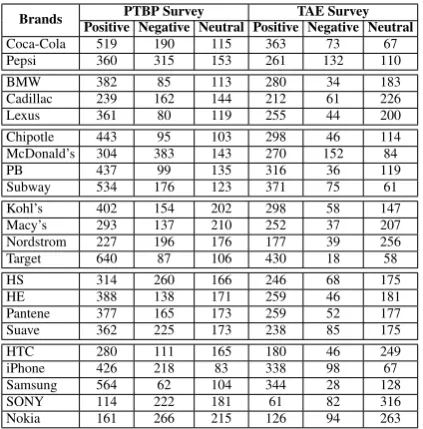
4.1 Definition and Statistics

For each brand in this study, we define people who havepositiveopinions as those who gave aloveor

likerating in their brand preference surveys. Simi-larly, people who havenegativeopinions are those who gave ahateordislikerating. People who gave aneutralrating are in theneutralcategory. Table 6 shows the number of instances in each of the three categories for each brand.

4.2 Classification

Brands _{Positive Negative Neutral Positive Negative Neutral}PTBP Survey TAE Survey

Coca-Cola 519 190 115 363 73 67 Pepsi 360 315 153 261 132 110 BMW 382 85 113 280 34 183 Cadillac 239 162 144 212 61 226 Lexus 361 80 119 255 44 200 Chipotle 443 95 103 298 46 114 McDonald’s 304 383 143 270 152 84 PB 437 99 135 316 36 119 Subway 534 176 123 371 75 61 Kohl’s 402 154 202 298 58 147 Macy’s 293 137 210 252 37 207 Nordstrom 227 196 176 177 39 256 Target 640 87 106 430 18 58 HS 314 260 166 246 68 175 HE 388 138 171 259 46 181 Pantene 377 165 173 259 52 177 Suave 362 225 173 238 85 175 HTC 280 111 165 180 46 249 iPhone 426 218 83 338 98 67 Samsung 564 62 104 344 28 128 SONY 114 222 181 61 82 316 Nokia 161 266 215 126 94 263

Table 6: Number of instances in each category

et al., 2009). Since our current goal is not to build the best brand preference prediction system, but to show the feasibility of building brand preference prediction systems that are scalable to millions of users, we ran all our classifiers using the default parameter settings from Weka (E.g. for Random Forest, we used 10 trees. The umber of features was set to log2(number of all features)+1.). We expect in the future, by optimizing model parame-ters, we can further improve the prediction power of each model.

The baseline classifiers classify every data in-stance into the majority class. Among all the classifiers we tested, we found that overall Naive Bayes has the best performance on both the PTBP and the TAE datasets. In the following, we report the average F-scores and AUC across 22 different brands using Naive Bayes with 10-fold cross val-idations. We created models that use all the user features and also those that use only trait features. Table 7 shows the results.

Best

Classifier FPTBPAUC F TAEAUC

All features 0.483 0.569 0.501 0.547

Traits only 0.475 0.556 0.502 0.528

Baseline 0.396 0.493 0.444 0.490

Table 7: 3-Way Classification Results

Overall, all the classifiers performed signifi-cantly better than the baselines (p<0.05). More-over, the models using all the features performed similarly to those using only trait features. The differences are not statistically significant. In ad-dition, comparing the models trained on the PTBP

data with those on the TAE dataset, their perfor-mances are very similar, although the exact num-bers are not directly comparable since they are from two different datasets.

To break down the results by product category, in Table 8, we list the per-brand classification re-sults using only the trait features. The numbers in the parentheses show the F-score percentage in-crease from the baselines. In general, models with trait features did much better than the baselines on both datasets. But their effectiveness varied from one brand to another. For example, the trait fea-tures were very effective in predicting user prefer-ences forCadillac (50.8% increase on the PTBP dataset and 68.5% increase on the TAE dataset). In contrast, there was barely any improvement for

Target. After inspecting the data, it seems this may be caused by the distribution of the data. For instance, the Target TAE data was very skewed. There were 430 people who had positive opinions about Target versus 18 people who had negative opinions. Since the baseline predicts “all people like Target”, which resulted in a pretty high F-score (0.781), any further improvement over this baseline became more difficult.

Brand _{BL F Best F}PTBP _{↑% BL F Best F}TAE _↑%

Coca-Cola 0.487 0.503 3.3% 0.605 0.605 0.0% Pepsi 0.263 0.427 62.4% 0.355 0.416 17.2% BMW 0.522 0.562 7.7% 0.406 0.499 22.9% Cadillac 0.266 0.401 50.8% 0.282 0.474 68.1% Lexus 0.505 0.531 5.2% 0.346 0.5 44.5% Chipotle 0.564 0.59 4.6% 0.513 0.53 3.3% McDonald’s 0.291 0.42 44.3% 0.371 0.459 23.7% PB 0.513 0.528 2.9% 0.539 0.58 7.6% Subway 0.501 0.525 4.8% 0.618 0.623 0.8% Kohl’s 0.368 0.466 26.6% 0.441 0.506 14.7% Macy’s 0.288 0.465 61.5% 0.342 0.5 46.2% Nordstrom 0.207 0.421 103.4% 0.381 0.467 22.6% Target 0.668 0.67 0.3% 0.781 0.781 0.0% HS 0.253 0.399 57.7% 0.337 0.454 34.7% HE 0.397 0.43 8.3% 0.371 0.494 33.2% Pantene 0.363 0.452 24.5% 0.368 0.51 38.6% Suave 0.307 0.375 22.2% 0.309 0.434 40.5% HTC 0.337 0.411 22.0% 0.361 0.455 26.0% iPhone 0.432 0.501 16.0% 0.54 0.557 3.2% Samsung 0.673 0.673 0.0% 0.561 0.574 2.3% SONY 0.258 0.407 57.8% 0.561 0.575 2.5% Nokia 0.243 0.397 63.4% 0.384 0.432 12.5%

Table 8: Classification Results By Brand

it implies that it is possible to build large-scale brand preference prediction systems that do not re-quire costly psychometric surveys.

4.3 Top Features

In this study, we want to find out what are the most significant features that can be used to differenti-ate a brand’s likers from dislikers. The feature se-lection was conducted using logistic regression in SPSS3_{. Due to the page limit, we cannot list all the}

significant features for all the 22 brands. Here we only show the most important features in predict-ing people who like and dislike luxury car brands based on the PTBP dataset (Table 9). Based on the regression analysis, all the features are sig-nificantly associated with brand preferences ( p< 0.05). In this table, personal trait features are high-lighted and followed by their types: P ( Personali-ties), V (Values), and N (Needs). “+” or “-” means the features contribute positively or negatively to the model. As shown in the table, more than half of all the top features are trait features. For ex-ample, the No. one trait feature to differentiate BMW likers from dislikers isideal, a trait associ-ated with people who have a desire for perfection. For Cadillac, the top trait is hedonism, which is often associated with people who pursue pleasure and sensuous gratification in life. For Lexus, the most useful feature isself-expression, a trait often associated with people who have a desire to assert their own identifies. Other interesting findings in-clude that females are less likely to be a fan of a luxury car brand than males. This is true across all three luxury car brands.

BMW Cadillac Lexus

ideal (N) + have children(no) - sports +

love (N) + television + self expression (N) +

conscientiousness (P) + hedonism (V) + television + gender(female) - home garden - self enhancement (V) + us news + gender(female) - fashion style + health + conservation (V) + theater

-hedonism (V) - self enhancement (V) - agreeableness (P) +

challenge (N) - science + openness to change (V)

-conservation (V) - love (N) - curiosity (N) +

self enhancement (V) + theater - gender(female)

-Table 9: Top 10 features for predicting opinions toward cars

5 Experiment 2

In the previous section, we demonstrated that given a particular brand such as Pepsi, it is possi-ble to automatically differentiate the people who have positive, negative or neutral opinions. In

3_{http://www-01.ibm.com/software/analytics/spss/}

this section, we try to answer a different question: given a list of competing brands in the same prod-uct category, can we automatically rank a user’s preferences of these brands? For example, given popular beverage brands such as Pepsi and Coca-Cola, can we automatically predict whether a per-son will like Pepsi or Coca-Cola more?

5.1 Average Rank for Each Brand

For each user, we rank all the brands in each prod-uct category based on his preferences in the sur-vey (e.g., 1 means most preferred brand). We ag-gregate the ranks from all the users and show the overall brand preference ranks for both datasets. As shown in table 10, the overall brand preference ranks for the PTBP and TAE surveys are highly correlated. Half of the product categories have ex-act the same preference ranks for all the products; The other half has only one slightly mis-matched rank in each product category. This suggests that the population participated in the PTBP and TAE survey has very similar brand preference distribu-tions. In the future, it maybe interesting to inves-tigate how this rank is related to different brands’ market share.

PTBP TAE

Beverage 1. Coca-cola_{2. Pepsi} 1. Coca-cola_{2. Pepsi}

Car 1. BMW2. Lexus 1. BMW2. Lexus 3. Cadillac 3. Cadillac

Fast Food

1. Chipotle 1. Panera Bread 2. Panera Bread 2. Chipotle 3. Subway 3. Subway 4. McDonald’s 4. McDonald’s

Retail

1. Target 1. Target 2. Macy’s 2. Kohl’s 3. Kohl’s 3. Macy’s 4. Nordstrom 4. Nordstrom

Shampoo

1. Herbal Essences 1. Herbal Essences 2. Pantene 2. Pantene 3. Suave 3. Head & Shoulders 4. Head & Shoulders 4. Suave

Smart Phone

1. Samsung 1. Samsung 2. iPhone 2. iPhone 3. HTC 3. HTC 4. Nokia 4. Nokia 5. SONY 5. SONY

Table 10: Overall preference rank

5.2 Rank Correlation

two types of models, one used all the user features, the other used traits only. We applied them to both the PTBP and the TAE datasets.

Since our model and the ground truth both pro-duce a ranked list for each product category, here we used rank correlation analysis to evaluate the quality of the predicted ranks. For each user and each product category, we computed the Spear-man’s rank correlation coefficient ρ. If the coef-ficientρis 1, there is a perfect positive correlation between the predict rank and the ground truth (i.e. both produce identical ranks). Ifρis -1, there is a perfect negative correlation between the predicted rank and the ground truth (i.e., the rank predicted by the system is exactly the opposite of the ground truth). If ρis 0 , then the predicted rank and the ground truth are randomly related. For each prod-uct category, we report the averageρacross all the users.

PTBP TAE

All Features Traits Only All Features Traits Only

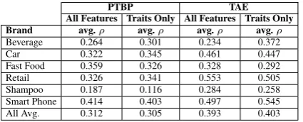
Brand avg.ρ avg.ρ avg.ρ avg.ρ

Beverage 0.264 0.301 0.234 0.372 Car 0.322 0.345 0.461 0.447 Fast Food 0.359 0.326 0.328 0.292 Retail 0.326 0.341 0.553 0.505 Shampoo 0.187 0.116 0.284 0.258 Smart Phone 0.414 0.403 0.497 0.545 All Avg. 0.312 0.305 0.393 0.403

Table 11: Evaluating predicted ranks

We use the overall rank data in Table 10 as our baseline. Specifically, for each product category, the baseline always ranks all its brands based on the average ranks defined in Table 10. For each user and each product category, we compute theρ between the user’s ground truth rank in the survey and the rank produced by the baseline. We com-pute the averageρ across all the users and all the product categories to represent the baseline perfor-mance. For the PTBP data, the average ρfor the baseline is 0.193. For the TAE data, the averageρ is 0.060.

There are several main findings from these re-sults. First, for all the product categories, the predicted ranks are all significantly and positively correlated with the ground truth (p <0.05). Also, our models perform significantly better than the non-personalized ranks produced by the baseline. This result is important because it shows that there is a stable and statistically significant agreement between the predicted ranks and the ground truth and the personalized models with additional trait features perform significantly better than the

non-personalized baseline system (on PTBP, the aver-age ρ of the model with personal traits is 0.305 versus 0.193 of the baseline. It is 0.403 versus 0.060 on the TAE dataset). Second, the perfor-mance on the TAE dataset is better than that on the PTBP dataset (e.g., the averageρ is 0.403 on TAE versus 0.305 on PTBP when only trait fea-tures were used). This may be due to the fact that in the TAE dataset, in addition to the Big 5 person-ality features, we also automatically extracted 30 personality sub-facets from tweets using the pro-cedure described in (Yarkoni, 2010). These finer-grained personality features are not available in the PTBP dataset. This result is encouraging since it suggests that using automatically inferred traits can predict brand preferences as well as if not bet-ter than the clean trait features that can be obtained only through costly psychometric evaluations. Fi-nally, for our models, since the overall correlation coefficientsρare between 0.3 and 0.4, the strength of these correlations is moderate. Thus, it may not be sufficient to build an accurate brand pref-erence prediction system with only user features. Other features especially brand-related features as well as features that capture the compatibility of a brand and a user are needed.

5.3 Top Features

We used multinomial logistic regression to find the most significant predicting features for each brand category. We show the feature ranks by signifi-cance for survey data in Table 12 and 13. Almost all of the top 10 features for each brand are signif-icantly correlated with the ranks. Again, the per-sonal traits features are highlighted and followed by their types: P (Personalities), V (Values), and N (Needs).

6 Conclusion and Future Direction

Beverage Car Fast Food

practicality (N) self enhancement (V) education status us news hedonism (V) gender

stability (N) television conservation (V)

science sports sports

curiosity (N) ideal (N) video games have children agreeableness (P) marital status

agreeableness (P) excitement (N) science

love (N) gender age

books health automobiles

marital status dining wine business

Smart Phone Retail Shampoo

books stability (N) gender

ideal (N) structure (N) age dining wine automobiles openness (P) closeness (N) health movie have children international news education status income education structure (N)

television have children curiosity (N) self enhancement (V) practicality (N) openness to change (V)

marital status conservation (V) theater

automobiles gender self transcendence (V)

Table 12: Top 10 features for predicting rank cor-relation (PTBP)

Beverage Car Fast Food

activity level (P) altruism (P) friend count

immoderation (P) adventurousness (P) sympathy (P) altruism (P) hedonism (V) conservation (V) intellect (P) openness (P) all tweet count

cautiousness (P) trust (P) self efficacy (P) extraversion (P) artistic interests (P) stability (N) friendliness (P) sympathy (P) altruism (P) self discipline (P) morality (P) depression (P) openness (P) liberalism (P) liberty (N) closeness (N) listed count gregariousness (P)

Smart Phone Retail Shampoo

neuroticism (P) openness to change (V) cautiousness (P) openness (P) love (N) cooperation (P) achievement striving (P) immoderation (P) intellect (P) altruism (P) sympathy (P) self consciousness (P) anger (P) hedonism (V) morality (P) assertiveness (P) all tweet count harmony (N) cautiousness (P) activity level (P) activity level (P) depression (P) trust (P) vulnerability (P) dutifulness (P) cautiousness (P) immoderation (P) immoderation (P) liberty (N) openness (P)

Table 13: Top 10 features for predicting rank cor-relation (TAE)

a user’s preference of competing brands within a product category. Our findings demonstrated that it is possible to use personal traits in predicting a user’s brand preferences. Moreover, we have also shown that automatically inferred user fea-tures are good proxies for the clean trait feafea-tures that can be acquired only from costly psychome-tric surveys. This work may have significant im-pact on the field of brand preference analysis since this suggests that it is possible for businesses to build scalable marketing tools to identify and tar-get potential customers on social media.

Brand preference prediction is a hard problem. So far, we have focused primarily on user features. To further improve the prediction accuracy, in the future, we will extend our current study by incor-porating new features such as the properties of a brand as well social influence from people in one’s social network.

References

Jennifer L Aaker. 1997. Dimensions of brand person-ality. Journal of Marketing Research, pages 347– 356.

Frank M Bass and W Wayne Talarzyk. 1972. An atti-tude model for the study of brand preference. Jour-nal of Marketing Research, pages 93–96.

David M Blei, Andrew Y Ng, and Michael I Jordan. 2003. Latent dirichlet allocation. the Journal of ma-chine Learning research, 3:993–1022.

Leo Breiman. 2001. Random forests. Machine Learn-ing, 45(1):5–32.

Barbara Everitt Bryant and Jaesung Cha. 1996. Cross-ing the threshold. Marketing Research, 8(4):20–28. Margaret C Campbell and Ronald C Goodstein. 2001. The moderating effect of perceived risk on con-sumers evaluations of product incongruity: Prefer-ence for the norm. Journal of Consumer Research, 28(3):439–449.

Gregory S Carpenter and Kent Nakamoto. 1989. Con-sumer preference formation and pioneering advan-tage. Journal of Marketing Research, pages 285– 298.

Richard L Celsi and Jerry C Olson. 1988. The role of involvement in attention and comprehension pro-cesses. Journal of Consumer Research, pages 210– 224.

Arjun Chaudhuri and Morris B Holbrook. 2001. The chain of effects from brand trust and brand affect to brand performance: the role of brand loyalty. Jour-nal of Marketing, 65(2):81–93.

Jilin Chen, Gary Hsieh, Jalal U Mahmud, and Jeffrey Nichols. 2014. Understanding individuals’ personal values from social media word use. InProceedings of the 17th ACM conference on Computer supported cooperative work & social computing, pages 405– 414. ACM.

Carolyn L Costley and Merrie Brucks. 1992. Selective recall and information use in consumer preferences.

Journal of Consumer Research, pages 464–474. Kitty G Dickerson. 1982. Imported versus

us-produced apparel: Consumer views and buying patterns. Home Economics Research Journal, 10(3):241–252.

Vytautas Dikcius, Eleonora Seimiene, and Ermita Za-liene. 2013. Congruence between brand and con-sumer personalities. Economic and Management, 18(3):526–536.

Richard Elliott. 1994. Exploring the symbolic mean-ing of brands. British Journal of Management, 5(s1):S13–S19.

Franklin B Evans. 1959. Psychological and objective factors in the prediction of brand choice ford versus chevrolet. The Journal of Business, 32(4):340–369. J Kevin Ford. 2005. Brands Laid Bare: Using Market

Research for Evidence-based Brand Management. John Wiley & Sons.

Yoav Freund and Robert E Schapire. 1996. Experi-ments with a new boosting algorithm. InThirteenth International Conference on Machine Learning, vol-ume 96, pages 148–156.

Lewis R Goldberg. 1993. The structure of phenotypic personality traits. American Psychologist, 48(1):26. Timothy R Graeff. 1996. Using promotional messages to manage the effects of brand and self-image on brand evaluations. Journal of Consumer Marketing, 13(3):4–18.

Russell I Haley and Peter B Case. 1979. Testing thir-teen attitude scales for agreement and brand discrim-ination. The Journal of Marketing, pages 20–32. Mark Hall, Eibe Frank, Geoffrey Holmes, Bernhard

Pfahringer, Peter Reutemann, and Ian H Witten. 2009. The weka data mining software: an update.

ACM SIGKDD explorations newsletter, 11(1):10– 18.

C Min Han and Vern Terpstra. 1988. Country-of-origin effects for uni-national and bi-national prod-ucts. Journal of International Business Studies, pages 235–255.

Phillip K Hellier, Gus M Geursen, Rodney A Carr, and John A Rickard. 2003. Customer repurchase inten-tion: a general structural equation model. European Journal of Marketing, 37(11/12):1762–1800. Jacob B Hirsh, Sonia K Kang, and Galen V

Boden-hausen. 2012. Personalized persuasion tailoring persuasive appeals to recipients personality traits.

Psychological Science, 23(6):578–581.

J Wesley Hutchinson, Kalyan Raman, and Murali K Mantrala. 1994. Finding choice alternatives in memory: Probability models of brand name recall.

Journal of Marketing Research, pages 441–461. Ahmad Jamal and Mark MH Goode. 2001. Consumers

and brands: a study of the impact of self-image con-gruence on brand preference and satisfaction. Mar-keting Intelligence & Planning, 19(7):482–492. Jong Soo Kim, Ming Hao Yang, Young Jin Hwang,

Sang Hoon Jeon, KY Kim, IS Jung, Chi-Hawn Choi, Wan-Sup Cho, and JH Na. 2012. Customer prefer-ence analysis based on sns data. InCloud and Green Computing (CGC), 2012 Second International Con-ference on, pages 609–613. IEEE.

Richard R Klink. 2001. Creating meaningful new brand names: A study of semantics and sound sym-bolism. Journal of Marketing Theory and Practice, pages 27–34.

Arthur Koponen. 1960. Personality characteristics of purchasers.Journal of Advertising Research.

Chin-Feng Lin. 2002. Segmenting customer brand preference: demographic or psychographic. Journal of Product & Brand Management, 11(4):249–268.

Kun Liu and Lei Tang. 2011. Large-scale behav-ioral targeting with a social twist. InProceedings of the 20th ACM international conference on Informa-tion and knowledge management, pages 1815–1824. ACM.

Vikas Mittal and Wagner A Kamakura. 2001. Sat-isfaction, repurchase intent, and repurchase behav-ior: investigating the moderating effect of customer characteristics. Journal of Marketing Research, 38(1):131–142.

Mohamed M Mostafa. 2013. More than words: Social networks text mining for consumer brand sentiments. Expert Systems with Applications, 40(10):4241–4251.

Nils Myszkowski and Martin Storme. 2012. How personality traits predict design-driven consumer choices. Europes Journal of Psychology, 8(4):641– 650.

JAF Nicholls, Sydney Roslow, and Henry A Laskey. 2011. Sports event sponsorship for brand promo-tion. Journal of Applied Business Research (JABR), 10(4):35–40.

Svein Ottar Olsen. 2002. Comparative evaluation and the relationship between quality, satisfaction, and re-purchase loyalty. Journal of the Academy of Market-ing Science, 30(3):240–249.

Nicolas Papadopoulos, Louise A Heslop, and Gary Bamossy. 1990. A comparative image analysis of domestic versus imported products. International Journal of Research in Marketing, 7(4):283–294.

Marco Pennacchiotti and Siva Gurumurthy. 2011. In-vestigating topic models for social media user rec-ommendation. InProceedings of the 20th interna-tional conference companion on World wide web, pages 101–102. ACM.

James W Pennebaker, Martha E Francis, and Roger J Booth. 2001. Linguistic inquiry and word count: Liwc 2001. Mahway: Lawrence Erlbaum Asso-ciates, 71:2001.

John C Platt. 1999. Fast training of support vector machines using sequential minimal optimization. In

Advances in kernel methods, pages 185–208. MIT press.

John Ross Quinlan. 1993. C4. 5: programs for ma-chine learning, volume 1. Morgan kaufmann. Shalom H Schwartz. 2003. A proposal for

measur-ing value orientations across nations.Questionnaire Package of the European Social Survey, pages 259– 290.

Janjaap Semeijn, Allard CR Van Riel, and A Beat-riz Ambrosini. 2004. Consumer evaluations of store brands: effects of store image and product at-tributes. Journal of Retailing and Consumer Ser-vices, 11(4):247–258.

Matthew D Shank and Lynn Langmeyer. 1994. Does personality influence brand image? The Journal of Psychology, 128(2):157–164.

Robert J Sutton and Peter C Riesz. 1979. The effect of product visibility upon the relationship between price and quality. Zeitschrift f¨ur Verbraucherpolitik, 3(2):145–150.

Richard Thaler. 1985. Mental accounting and con-sumer choice. Marketing Science, 4(3):199–214. Yann Truong, Rod McColl, and Philip J Kitchen. 2010.

Uncovering the relationships between aspirations and luxury brand preference. Journal of Product & Brand Management, 19(5):346–355.

David K Tse and Gerald J Gorn. 1993. An experi-ment on the salience of country-of-origin in the era of global brands. Journal of International Market-ing, pages 57–76.

B¨ulent ¨Ust¨un, Willem J Melssen, and Lutgarde MC Buydens. 2006. Facilitating the application of sup-port vector regression by using a universal pearson vii function based kernel. Chemometrics and Intel-ligent Laboratory Systems, 81(1):29–40.

William Yang Wang, Edward Lin, and John Kominek. 2013. This text has the scent of starbucks: A lapla-cian structured sparsity model for computational branding analytics. InProceedings of the 2013 Con-ference on Empirical Methods in Natural Language Processing (EMNLP 2013), Seattle, WA, USA. Ralph Westfall. 1962. Psychological factors in

pre-dicting product choice. The Journal of Marketing, pages 34–40.

Robert E Witt and Grady D Bruce. 1972. Group influ-ence and brand choice congruinflu-ence. Journal of Mar-keting Research, pages 440–443.

Wendy Wood and Timothy Hayes. 2012. Social influ-ence on consumer decisions: Motives, modes, and consequences. Journal of Consumer Psychology, 22(3):324–328.

Huahai Yang and Yunyao Li. 2013. Identifying user needs from social media. Technical report, IBM Tech Report. goo. gl/2XB7NY.

Tal Yarkoni. 2010. Personality in 100,000 words: A large-scale analysis of personality and word use among bloggers. Journal of Research in Personal-ity, 44(3):363–373.