Evaluation of Rhodotorula growth on solid substrate via a linear mixed effects model

Evaluation of

Rhodotorula

Growth on Solid Substrate

via

a Linear Mixed Effects Model

Tereza KRuliKoVSKá

_{, Eva JaRošoVá}

_{and Petra PaTáKoVá}

1_{Department of Fermentation Chemistry and Bioengineering, Faculty of Food and Biochemical}

Technology, institute of Chemical Technology Prague, Prague, Czech Republic; 2_{Skoda auto university, Mladá Boleslav, Czech Republic}

Abstract

Krulikovská T., Jarošová E., Patáková P. (2011): Evaluation of Rhodotorulagrowth on solid substrate

via a linear mixed effects model. Czech J. Food Sci., 29: 400–410.

The growth of Rhodotorula glutinis and Rhodotorula mucilaginosa was studied under optimal and stress cultivation conditions at 10°C and 20°C for 14 days. The method of image analysis was used to determine the size of colonies. The linear mixed effects model implemented in the statistical program S-PLUS was applied to analyse the repeated measure-ments. Two-phase kinetics was confirmed and the mean growth rates in the second linear phase under various stress conditions were estimated. The results indicated a higher growth rate of R. mucilaginosa than was that of R. glutinis under all cultivation conditions. The highest growth rate of was observed during the cultivation of R. mucilaginosa in media with 2% of NaCl at 20°C. The impact of neglecting the fact that repeated data are not independent and using the classical regression model instead of the mixed effects model was demonstrated through the comparison of the confidence intervals for the parameters based on both approaches. While the point estimates of the corresponding parameters were similar, the width of the confidence intervals differed substantially.

Keywords: confidence intervals; giant colony; growth curves; image analysis; solid substrate cultivation

Supported by the Ministry of Education, Youth and Sports of the Czech Republic, Project No. MSM 6046137305.

Rhodotorula belongs to a genus of imperfect

yeasts, is well known as a producer of carotenoid pigments, and has both positive and negative sig-nificance in agriculture and food industry (Yeeh 2000). Its ability to suppress the growth and patu-lin production of Penicillium expansum makes it a potential good biocontrol agent usable for the reduction of postharvest decay of apples (Cas-toria et al. 2005) or pears (Zhang et al. 2008). This Rhodotorula use could increase the safety of fruit products like juices. At the same time,

Rho-dotorula belongs to food contaminants (cheese,

fruit, fruit juices and meat products) (Viljoen & Greyling 1995; Yeeh 2000; Restucciaet al. 2006). Rhodotorula was chosen for our experiments for its advantageous features: pseudomycelium

is formed occasionally; colonies are smooth with clearly defined boundaries (Yeeh 2000). Until now, the main interest in the literature has been concentrated on Saccharomyces cerevisiae; there is still a lack of information about the behaviour

of Rhodotorula.

The growth of giant colonies of yeast on agar plates may be regarded as the simplest example of solid substrate cultivation (Mitchel 1992b).

Several models of the growth of yeasts or fungi on solid substrates have been presented in the lit-erature (Pirt 1967). These models are based on the measurement of biomass or colony diameter (Valik & Pieckova 2001; Hamidi-Esfahani et al. 2004; Marín et al. 2007). Direct biomass determination in most SSC is difficult due to the problems con-nected with the separation of the organism from the substrate. Even indirect methods of biomass estimation (e.g. monitoring of metabolic activities) cannot be always applied (Mitchel 1992a; Araya et al. 2007).The colony diameter is usually measured several times in horizontal and vertical directions which is very inaccurate and time consuming. The modern method of image analysis can be used in-stead (Vecht-Lifshitz & Ison 1992; Thomas & Paul 1996; Couri et al. 2006).

A common way of analysis consists in modelling averages over different specimens exposed to the same experimental conditions. Because the true covariance structure of the data due to repeated observations of the specimens made over time is not taken into account, the inference is not quite correct. The mixed effects model can be used for the data where the observations of the same item are correlated and a higher correlation can be expected between adjacent observations than between those more distant in time. A detailed description of the mixed effects models (both lin-ear and nonlinlin-ear) can be found in Pinheiro and Bates (2000). The mixed effects model was used e.g. by Miguez et al. (2008) for the analysis of the growth curves of biomass crops or by Shorten

et al. (2004) as a tool for variance component

analysis in a microbial problem.

The aim of our study was to evaluate the growth

of Rhodotorula during SSC under various

cul-tivation conditions. The data were obtained by the image analysis and the linear mixed effects model was used for the analysis. To the best of our knowledge, Rhodotorula growth in SSC process has never been studied.

MATERIAL AND METHODS

Yeasts. Rhodotorula mucilaginosa (DBM 19)

was obtained from DBM-Culture Collection of the Department of Biochemistry and Microbiology,

Institute of Chemical Technology in Prague, Czech Republic. Rhodotorula glutinis (CCY 20-2-20) was obtained from CCY-Culture Collection of Yeasts, Slovak Academy of Sciences, Bratislava.

Inoculum preparation. The following liquid

medium was used for the yeast growth: glucose 25 g/l, yeast extract 10 g/l, K₂HPO₄ 2 g/l, KH₂PO₄ 2 g/l, MgSO₄·7H₂O 0.1 g/l; pH was adjusted to 6.0. The liquid media in Erlenmeyer flasks were inoculated with the yeast grown on agar slant. Shaken flasks (300 rpm) were incubated at 28°C for two days.

Giant colony cultivation. A drop of the cell

suspension was laid on Sabouraud’s agar (14 ml) in the middle of a Petri dish (Ø = 60 mm). Agar plates were inoculated with suspensions of young cells, which contained about 107_–109 _cells/ml. The plates were cultivated at 10°C or 20°C for approximately 14 days. NaCl (0%, 10%, and 2%) was used as exogenous osmotic stress factor. Low concentrations of the stress factor (NaCl, 1% or 2%) were chosen to ensure agar solidification. Two temperatures were chosen according to Bhosale and Gadre (2002) who described significant dif-ferences in total carotene pigment concentration during cultivation at 10°C and 20°C. Six specimens under the same treatment conditions were observed at one-day intervals.

Measurement of giant colony size. The colony

growth was measured by the method of image analysis. The photos of the colonies were taken by the digital camera FinePix S7000 (Fujifilm, Japan). The camera was fixed on a Kaiser RS1 (support with Kaiser RB 5000 DL (Germany) illuminating system. Image processing procedures were done in software Lucia (Laboratory Imaging Ltd., Prague, Czech Republic). A simple macro was created for photo evaluation.

An appropriate threshold was used for the ob-ject separation from the background. Afterwards, mathematical operations such as clean, close and fill-holes were applied to produce the final binary image. The area of the colony and other param-eters were measured. In one of the treatments, the consistency of the automatically determined results (macro) was checked by manual measure-ment. A high degree of correlation (0.999, sample size 56, P < 0.0001) was confirmed.

Software. Sigma Stat software (version 3.1) and

Growth model. The equivalent colony diameter, i.e. the diameter of a circle having the same area as the colony was chosen as a response variable. In matrix notation, the linear mixed effects model is written as

y = Xβ + Zb + e (1)

where:

y – vector of responses

X – known design matrix linking β to y

β – vector of unknown parameters (fixed effects) Z – design matrix linking b to y

b – vector of unknown random effects e – vector of random errors.

Assuming b ~ N(0,D), e ~ N(0,R), and b and e being independent, the mean profile is given by E(y) = Xβ and the covariance structure depends on the matrices D and R, namely var(y)= ZDZT _{+ R.}

With time taken as continuous and on the as-sumption that our measurements record the pe-riod of the linear growth (Pirt 1967) where the starting time point is t₀, the colony diameter of the i-th specimen at the j-th level of temperature, the k-th level of NaCl concentration, and time t_l is expressed in the form:

y_ijkl = β_0,jk + b_0,i) + (β_1,jk + b_1,i)(t_l – t₀) + e_ijkl (2)

(i = 1, 2, ..., 36; j = 1, 2; k = 1, 2, 3; l = 1, 2, ..., 288 in our study)

where:

β_0,jk – corresponds to the mean diameter at t = t₀

β_1,jk – mean growth rate (in cm per day) in the “linear” period

b_0,i – amount by which the “intercept” of the i-th straight line differs from β_0,jk

b_1,i – difference between the slope of the i-th straight line and β_1,jk

The random variables b₀ and b₁ are called ran-dom effects and their variations across different specimens are described by parameters σ₀2 _and σ₁2_{,respectively. These parameters lie on the main} diagonal of D (2 × 2). In a special case of uncor-related b₀ and b₁, D is a diagonal matrix. A more general covariance model with heterogeneous varia-tion of random effects across different experimental conditions may be considered; in that case, D will have a larger dimension. Random errors e_ijkl denote the departures of observations from the model. In the case of independence and homoscedasticity, their covariance matrix would be R = σ2_{I. When}

the growth curves are analysed, often the autore-gressive scheme AR(1) is considered (the model e_t = Φ e_t–1 + ν_t, where Φ is an autocorrelation coef-ficient and random component v_t has the properties of the white noise, see e.g. Pinheiro & Bates 2000). This special form of R is described by two parameters; σ denotes standard deviation of the error component ν_t, Φ is the autocorrelation coefficient.

It follows that the linear mixed effects model has both the mean structure and the covariance struc-ture. The mean profile representing the growth under the specific treatment conditions has the form:

E(y) = β_0,jk + β_1,jk (t – t₀) (3) The indices j and k stand for the j-th level of tem-perature and the k-th level of NaCl concentration. Both parameters are supposed to be affected by the treat-ment (note that β_0,jk does not represent the intercept at t = 0 but t₀ = 5). In fact, β_0,jk and β_1,jk are the sums of several fixed-effects parameters depending on which fixed effects are included in the model. The covariance structure is described by matrices D and R.

The fixed-effects parameters and covariance parameters of the selected structures are usually estimated by the maximum likelihood method or by the restricted maximum likelihood method, see e.g. Pinheiro and Bates (2000). Here the latter was used. During the model building, conditional t-tests are applied to test the significance of the fixed-effects parameters, and the information criteria AIC and BIC (see e.g. Pinheiro & Bates 2000) are used to find appropriate forms of D and R. Besides, the checking of confidence intervals for covariance parameters in D and R is recom-mended by Pinheiro and Bates (20006).

Approximate confidence intervals for β_0,jk are given by

βˆ_0,jk ± t_1–α/2,ν σˆ (βˆ_0,jk) (4) where:

βˆ_0,jk – denotes the estimates of β_0,jk

t_1–α/2,ν – 1–α/2 quantile of the i-distribution with ν degrees of freedom

σˆ(βˆ_0,jk) – denotes the estimate of the standard error of βˆ_0,jk Similarly for the confidence intervals for β_0,jk.

Remark: The terms conditionalt-tests and approximate

Table 1. Estimated covariance parameters for R. glutinis (procedure lme, S-PLUS)

Matrix D Matrix R

σˆσ₀ ˆσ ˆΦ

0.0477 0.0182 0.6986

σˆσ₀ – standard deviation of b₀; σˆσ– error standard deviation; ˆΦ – autocorrelation coefficient

RESULTS

The camera and illuminating systems used in the experiment did not enable us to monitor the initial stages of the colony growth due to a low contrast between the colony and the background (agar plates). The first results were obtained after five days. From then on, most growth curves ex-hibited linear dependence of equivalent diameter on time (Figure 1).

The data for the two Rhodotorula species were analysed separately. The observations on speci-mens No. 19 (Figure 1e) and No. 31 (Figure 1f ) of

R. glutinis, the growth curves of which differed

strikingly from those obtained under the same treatment, were excluded from the analysis.

Rhodotorula glutinis

Parallel lines under the same treatment con-ditions suggested that only the random effects b₀, representing the variation around β_0,jk, were needed in the model and D was reduced to scalar σ₀2_. The matrix R corresponded to the autoregressive scheme AR(1). The estimates of the corresponding parameters are shown in Table 1.

The variation of random effects b₀ described by σ₀2 _{might have been caused either by different} initial conditions of the individual specimens or by random variation of the growth rates in the initial period. Owing to the fact that the growth rates of all specimens under the same treatment conditions in the following period were practi-cally the same, the former cause seemed to be more probable.

The estimates of the fixed-effects parameters are displayed in Table 2. Both the main effects and interaction effects were included in the model. The parameters were estimated by the procedure lme in S-PLUS.

Using these estimates and their approximate covariance matrix provided by lme in S-PLUS (not displayed), the estimates of β_0,jk and β_1,jk including

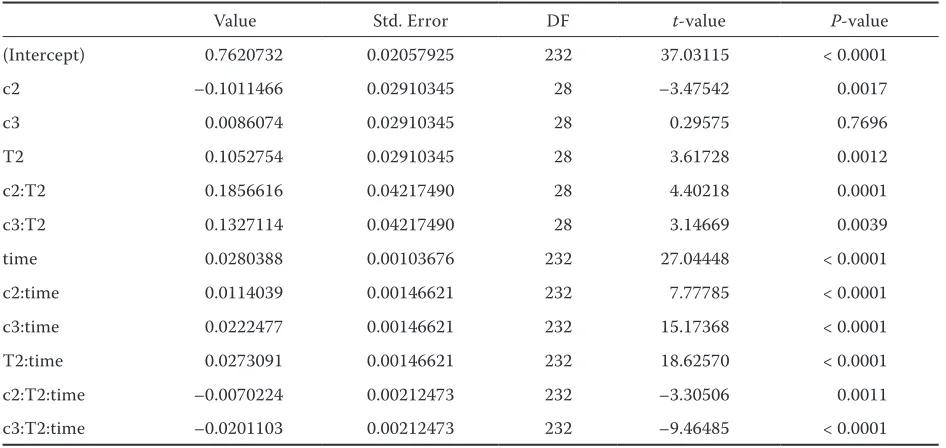
Table 2. Estimated fixed-effects parameters for R. glutinis (the output of lme, S-PLUS)

Value Std. Error DF t-value P-value

(Intercept) 0.7620732 0.02057925 232 37.03115 < 0.0001

c2 –0.1011466 0.02910345 28 –3.47542 0.0017

c3 0.0086074 0.02910345 28 0.29575 0.7696

T2 0.1052754 0.02910345 28 3.61728 0.0012

c2:T2 0.1856616 0.04217490 28 4.40218 0.0001

c3:T2 0.1327114 0.04217490 28 3.14669 0.0039

time 0.0280388 0.00103676 232 27.04448 < 0.0001

c2:time 0.0114039 0.00146621 232 7.77785 < 0.0001

c3:time 0.0222477 0.00146621 232 15.17368 < 0.0001

T2:time 0.0273091 0.00146621 232 18.62570 < 0.0001

c2:T2:time –0.0070224 0.00212473 232 –3.30506 0.0011

c3:T2:time –0.0201103 0.00212473 232 –9.46485 < 0.0001

c2 (c3) – 2nd ₍₃rd_{) level of NaCl concentration; T2 – 2}nd _{level of temperature, time is a continuous variable}

The estimated fixed-effects parameters in the 2nd _{column are used to compute βˆ}

Figure 1. Growth curves of Rhodotorula giant colonies. Rhodotorula glutinis (RG) and Rhodotorula mucilaginosa

(RM) were cultivated on Sabouraud agar plates at 10°C or 20°C for 14 days. Different NaCl concentrations (0%, 1%, and 2%) were added to the media as a stress factor. First results were observed after 5 days

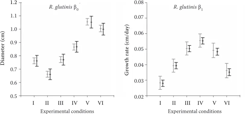
conventional confidence limits were computed (Table 3) and displayed (Figure 2).

In general, the temperature and concentration af-fect both the mean diameter β_0,jk at t₀ and the mean growth rate β_1,jk. The significance of the individual terms can be checked through P-values. It can be said that the temperature had a positive effect

on β_0,jk and β_1,jk. Due to the fact that there were three levels of concentration in the experiment, we could observe a nonlinear effect of concentra-tion on βˆ_0,jk in the range 0–2%. The impact of the interaction of the temperature and concentration can be seen best in Figure 2 where the interval midpoints correspond to βˆ_0,jk or βˆ_1,jk.

Time (day) Time (day) Time (day)

Time (day) Time (day) Time (day)

Time (day) Time (day) Time (day)

Time (day) Time (day) Time (day)

Considering the same initial mean diameter regardless of the treatment as a reasonable as-sumption, the differences between the estimates βˆ_0,jk reflected different mean rates under various treatment conditions in the previous growth pe-riod.

Rhodotorula mucilaginosa

Although the growth lines at 20°C and 2% NaCl indicated a slight variation of slopes (Figure 1), only the random effects b₀ were included in the model based on the information criteria (see Model validation). The differences between σ₀ (standard deviations of random effects b₀) under different treatment conditions were apparent. The effects of both the temperature and concentration are distinguishable in Figure 1, however, based on

the information criteria, the form D = diag{σ₀2 ,1, σ₀2

,2, σ02,3}was chosen, where the three parameters corresponded to the three levels of NaCl concen-tration. The estimates of the standard deviations supplemented by the estimates of the matrix R parameters are given in Table 4. The estimates of the fixed-effects parameters are given in Table 5, the estimates of β_0,jk and β_1,jk including conventional confidence limits are displayed in Table 6.

Due to the positive signs of all estimated effects, the results were more straightforward than with

R. glutinis. Both the temperature and

concentra-tion had a positive effect on β_0,jk and β_1,jk (though insignificant in the case of concentration and β_0,jk) and the nonlinear effect of concentration almost did not exhibit. Again, the interaction of temperature and concentration affected both β_0,jk and β_1,jk significantly. The impact of the interac-tion can be detected in Figure 3.

Table 3. Estimated parameters of the straight lines with 95% confidence limits for R. glutinis

Experimental

conditions T (°C) c (%) βˆ1 95% lcl 95% ucl βˆ1 95% lcl 95% ucl

I 10 0 0.7621 0.7215 0.8026 0.0280 0.0260 0.0301

II 10 1 0.6609 0.6204 0.7015 0.0394 0.0374 0.0415

III 10 2 0.7707 0.7301 0.8112 0.0503 0.0482 0.0523

IV 20 0 0.8673 0.8268 0.9079 0.0553 0.0533 0.0574

V 20 1 1.0530 1.0086 1.0974 0.0483 0.0461 0.0506

VI 20 2 1.0001 0.9556 1.0445 0.0352 0.0330 0.0375

βˆ₀ – mean diameter after 5 days; βˆ₁– mean growth rate during the linear growth period

Figure 2. Confidence intervals for β₀ and β₁ based on LME (black bar) and LM (grey bar) under different experimental conditions, Rhodotorula glutinis

R. glutinis β₀ R. glutinis β₁

1.2

1.1

1.0

0.9

0.8

0.7

0.6

0.5

D

ia

m

et

er

(c

m

)

0.08

0.07

0.06

0.05

0.04

0.03

0.02

G

ro

w

th

ra

te

(c

m

/d

ay

)

I II III IV V VI I II III IV V VI

Model validation

The lack-of-fit test was performed to check the mean structure model as a linear function of time. Although P-values were only approximate in this case of the dependent data, the values of 0.999978 and 0.996675 for Rhodotorula glutinis and

Rhodo-torula mucilaginosa, respectively, clearly indicated

the fitness of the linear relationship.

Various forms of D (2 × 2 diagonal, 2 × 2 general, and various kinds of structures with heterogeneous variances) and two forms of R, i.e. AR(1) scheme or independent errors were examined. Only covariance models with diagonal D are involved in Tables 7 and 8 because either the restricted maximum likelihood method failed due to a large number of parameters or an infinitive confidence interval for off-diagonal parameters indicated a redundancy of the param-eters. As for R. glutinis (Table 7), AIC indicated RG1 and BIC indicated RG4 as the best model (the lower the values of AIC and BIC, the better). The criterion BIC penalising models with a greater number of

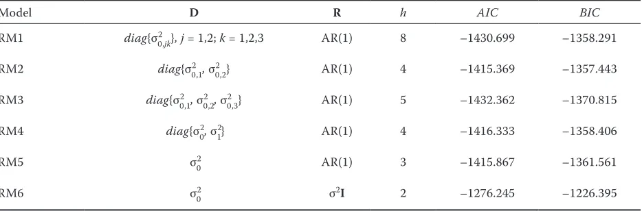
parameters was preferred. Another reason for the choice of RG4, the third best by AIC, was the fact that σ₀ did not appear to be dependent either on the temperature or on NaCl concentration. In the case of R. mucilaginosa,both criteria indicated RM3 as the best (Table 8)

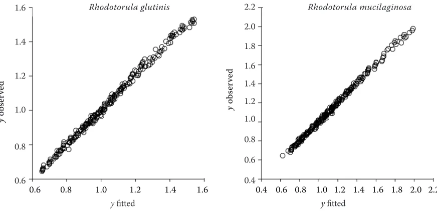
Q-Q plots (Figure 4) are nearly straight, indicat-ing no serious evidence against the assumption of normality. Plots in Figure 5 show a very good agreement between the observed data and the fitted model including random effects and may serve as a further confirmation of the adequacy of both the mean and the covariance structure models.

Besides the mixed effects model, the classical model was applied so that we could demonstrate the differences between the lengths of the confi-dence intervals obtained by the two approaches. All intervals are displayed in Figures 2 and 3. It is obvious that the corresponding estimates obtained by the two approaches did not differ essentially. But the differences in the lengths are striking, though expected. The length of the interval for β_0,jk based on the classical model is roughly half the length of the interval based on the mixed effects model, the opposite is true in the case of β_1,jk.

DISCUSSION

Although it was impossible to measure the area at the beginning of the process in our experiment, the data analysis indicated a two-phase kinetic profile. This was based on the fact that the intercepts of

Figure 3. Confidence intervals for β₀ and β₁ based on LME (black bar) and LM (grey bar) under different experimental conditions, Rhodotorula mucilaginosa

Table 4. Estimated covariance parameters for R. muci-laginosa (procedure lme, S-PLUS

Matrix D Matrix R

c (%) 0 1 2 _ˆσ ˆΦ

ˆσ 0.0126 0.0013 0.0629 0.0234 0.7998

ˆσ₀ – standard deviation of b₀dependent on NaCl concen-tration; ˆσ – error standard deviation; ˆΦ – autocorrelation coefficient

R.mucilaginosa β₀ R. mucilaginosa β₁

1.2

1.1

1.0

0.9

0.8

0.7

0.6

0.5

D

ia

m

et

er

(c

m

)

0.09

0.08

0.07

0.06

0.05

0.04

0.03

0.02

G

ro

w

th

ra

te

(c

m

/d

ay

)

I II III IV V VI I II III IV V VI

the growth lines obtained by extrapolation for t = 0 differed across the experimental treatments which contradicted the reasonable assumption that only random variation of the specimen sizes was possible at t = 0 because different experimental conditions could not yet manifest themselves. It followed that

the growth rate in the first phase before t₀ must have differed from the constant rate observed past t = t₀. This finding was not unexpected (Mitchel 1992b; Valik & Pieckova 2001).

Based on the estimates βˆ_0,jk reflecting the mean growth rate in the unobserved initial phase and

Figure 4. Q-Q plot to check on the assumption of normality (Standardised residuals correspond to the model includ-ing random effects)

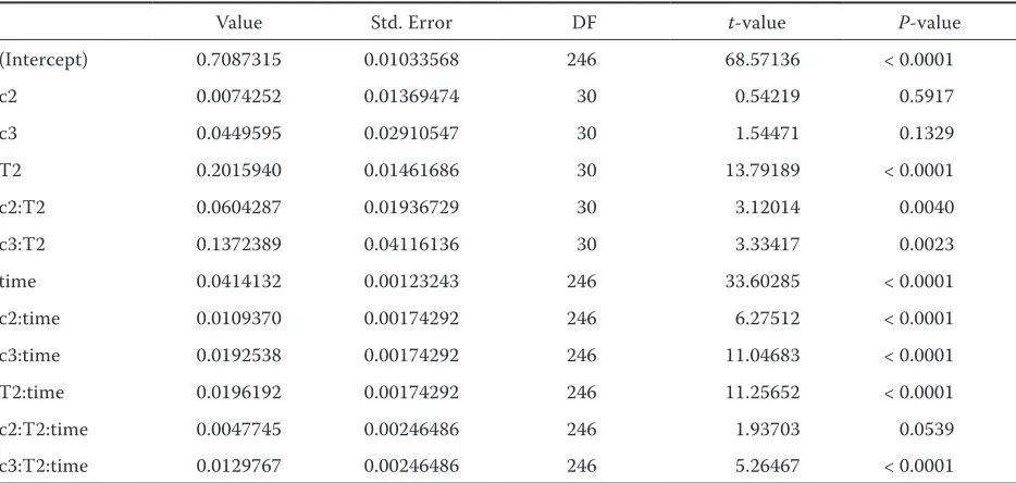
Table 5. Estimated fixed-effects parameters for R. mucilaginosa (lme, S-PLUS)

Value Std. Error DF t-value P-value

(Intercept) 0.7087315 0.01033568 246 68.57136 < 0.0001

c2 0.0074252 0.01369474 30 0.54219 0.5917

c3 0.0449595 0.02910547 30 1.54471 0.1329

T2 0.2015940 0.01461686 30 13.79189 < 0.0001

c2:T2 0.0604287 0.01936729 30 3.12014 0.0040

c3:T2 0.1372389 0.04116136 30 3.33417 0.0023

time 0.0414132 0.00123243 246 33.60285 < 0.0001

c2:time 0.0109370 0.00174292 246 6.27512 < 0.0001

c3:time 0.0192538 0.00174292 246 11.04683 < 0.0001

T2:time 0.0196192 0.00174292 246 11.25652 < 0.0001

c2:T2:time 0.0047745 0.00246486 246 1.93703 0.0539

c3:T2:time 0.0129767 0.00246486 246 5.26467 < 0.0001

c2 (c3) – 2nd ₍₃rd_{) level of NaCl concentration; T2 – 2}nd _{level of temperature, time is a continuous variable, time is a continuous}

variable

The estimated fixed-effects parameters in the 2nd _{column are used to compute βˆ}

0,jk and βˆ1,jk in Table 6. The value at Intercept corresponds to βˆ_0,11 at 10°C and 0% NaCl, the value at c2 (c3, T2) is added to obtain βˆ_0,12 (βˆ_0,13, βˆ_0,21), the value at c2:T2 (c3:T2) is a1dded together with those at c2 (c3) and T2 to obtain β_0,22 (β_0,23). The value at time corresponds to βˆ_0,11, i.e. to the growth rate at 10°C and 0% NaCl, the other values of βˆ_1,jk are obtained in a similar way as βˆ_0,jk

Rhodotorula glutinis Rhodotorula mucilaginosa

4

3

2

1

0

–1

–2

–3

–4

Q

ua

nt

ile

s o

f s

ta

nd

ar

d

no

rm

al

4

3

2

1

0

–1

–2

–3

–4

Q

ua

nt

ile

s o

f s

ta

nd

ar

d

no

rm

al

–3 –2 –1 0 1 2 3 –3 –2 –1 0 1 2 3

βˆ_1,jk representing the mean growth rates in the observed linear phase, it can be concluded that in the case of R. mucilaginosa both rates were positively affected by the temperature and NaCl concentration. As for R. glutinis, the results were not so straightforward. The positive effect of tem-perature existed in both phases of the growth with the exception of the highest NaCl concentration in the observed phase. The dependence on NaCl concentration was different both at the two tem-peratures and in the two phases. The reason can hardly be found due to the observations missing in the initial phase. The results clearly indicate that the growth rate of R. mucilaginosa was higher than that of R. glutinis under all cultivation conditions. The highest growth rate was observed during the cultivation of R. mucilaginosa in the media with 2%

of NaCl at 20°C. The covariance structures of the models describing SSC growth of the two yeasts were slightly different but this can be explained by the fact that the greater variation of b₀ comes about at the higher growth rate. This supposition is also supported by the larger variation around βˆ_0,jk at 20°C and 2% NaCl for R. glutinis (not considered in the model) and obviously a larger variation around βˆ_1,jk at 20°C and 2% NaCl for R. mucilaginosa (not considered in the model).

The use of the linear mixed effects model offers a more precise analysis than does the classical linear model. As shown in our paper, the impacts of neglecting assumptions of the classical linear model on the length of confidence intervals for the parameters of the model may be quite es-sential. The use of the model is not restricted to

Figure 5. Comparison of fitted and observed values of colony diameter. Fitted values correspond to the model includ-ing random effects, observed values are the response values

1.6

1.4

1.2

1.0

0.8

0.6

y

o

bs

er

ve

d

2.2

2.0 1.8

1.6 1.4 1.2 1.0

0.8

0.6

0.4

y

o

bs

er

ve

d

0.6 0.8 1.0 1.2 1.4 1.6 0.4 0.6 0.8 1.0 1.2 1.4 1.6 1.8 2.0 2.2

y fitted y fitted

Table 6. Estimated parameters of the of the straight lines with 95% confidence limits for R. mucilaginosa

Experimental

conditions T (°C) c (%) βˆ0 95% lcl 95% ucl βˆ1 95% lcl 95% ucl

I 10 0 0.7087 0.6682 0.7493 0.0414 0.0394 0.0435

II 10 1 0.7162 0.6756 0.7567 0.0524 0.0503 0.0544

III 10 2 0.7537 0.7132 0.7942 0.0607 0.0586 0.0627

IV 20 0 0.9103 0.8698 0.9509 0.0610 0.0590 0.0631

V 20 1 0.9708 0.9264 1.0152 0.0658 0.0636 0.0680

VI 20 2 1.0477 1.0033 1.0921 0.0740 0.0718 0.0762

βˆ₀ – mean diameter after 5 days; βˆ₁– growth rate during the linear growth period

the functions linear in parameters; non-linear mixed effects models are applied in a similar way. Both linear and non-linear mixed effects models are implemented in the best known commercial software products such as S-PLUS or SAS.

References

Araya M.M., Arrieta J.J., Peréz-Correa J.R., Biegler, L.T., Jorquera H. (2007): Fast and reliable calibration of solid substrate fermentation kinetics models using

Table 8. Covariance structure models specified by matrices D and R and corresponding information criteria AIC and BIC for R. mucilaginosa (lme, S-PLUS)

Model D R h aiC BiC

RM1 diag{σ₀2

,jk}, j = 1,2; k = 1,2,3 AR(1) 8 –1430.699 –1358.291

RM2 diag{σ₀2

,1, σ02,2} AR(1) 4 –1415.369 –1357.443

RM3 diag{σ₀2

,1, σ02,2, σ02,3} AR(1) 5 –1432.362 –1370.815

RM4 diag{σ₀2_{, σ}

12} AR(1) 4 –1416.333 –1358.406

RM5 σ₀2 _{AR(1) 3 –1415.867 –1361.561}

RM6 _σ02 _σ2_{I 2 –1276.245 –1226.395}

The covariance matrix of random effects D of model RM1 has six different variances σ₀2

,jk corresponding to the different experimental conditions on its diagonal. In RM2 σ₀2

,1, σ02,2 , correspond to different temperatures, in RM3 σ02,1, σ02,2, σ02,3,

correspond to different concentrations. In RM4 σ₀2 _{and σ} 1

2 _{and in RM5 and RM6 only σ}

02 independent on experimental

conditions is considered. The covariance matrix of random errors R corresponds either to the autoregressive scheme AR(1) or to the independent random errors with equal variances (I is the identity matrix). By h the overall number of covariance parameters in D and R is denoted

advanced non-linear programming techniques. Electronic Journal of Biotechnology, 10: 48–60.

Bhosale P., Gadre R.V. (2002): Manipulation of tempera-ture and illumination conditions for enhanced β-carotene production by mutant 32 of Rhodotorula glutinis. Letters in Applied Microbiology, 34: 349–353.

Castoria R., Morena V., Caputo L., Panfili G., De Cur-tis F., De Cicco V. (2005): Effect of the biocontrol yeast Rhodotorula glutinisstrain LS11 on patulin accumulation in stored apples. Phytopathology,95: 1271–1278. Couri S., Merces E.P., Neves B.C.V., Senna L.F. (2006):

Digital image processing as a tool to monitore biomass

Table 7. Covariance structure models specified by matrices D and R and corresponding information criteria AIC and BIC for R. glutinis (lme, S-PLUS)

Model D R h aiC BiC

RG1 diag{σ₀2

,jk}, j = 1,2; k = 1,2,3 AR(1) 8 –1356.121 –1284.908

RG2 diag{σ₀2

,1, σ02,2} AR(1) 4 –1346.230 –1289.259

RG3 diag{σ₀2

,1, σ02,2, σ02,3} AR(1) 5 –1346.520 –1285.988

RG4 σ₀2 _{AR(1) 3 –1347.683 –1294.273}

RG5 _σ02 _σ2_{I 2 –1276.245 –1226.395}

The covariance matrix of random effects D of model RG1 has six different variances σ₀2

,jk corresponding to the different experimental conditions on its diagonal. In RG2 σ₀2

,1, σ02,2, correspond to different temperatures, in RG3 σ02,1, σ02,2, σ02,3 ,

growth in aspergilus niger 3T5B8 solid-state fermenta-tion: preliminary results. Journal of Microscopy, 225: 290–297.

Hamidi-Esfahani Z., Shojaosadati S.A., Rinzema A. (2004): Modelling of simultaneous effect of moisture and temperature on a. niger growth in solid-state fermenta-tion. Biochemical Engineering Journal, 21: 265–272. Marín S., Cuevas D., Ramos A. J., Sanchis V. (2007):

Fitting of colony diameter and ergosterol as indicators of food borne mould growth to known growth models in solid medium. International Journal of Food Microbiol-ogy, 121: 139–149.

Miguez F.E., Villamil M.B., Long S.P., Bollero G.A. (2008): Meta-analysis of the effects of management fac-tors on Miscanthus × giganteus growth and biomass production. Agricultural and Forest Meteorology, 148: 1280–1292.

Mitchel D.A. (1992a): Biomass determination in solid-state cultivation. In: Doelle H.W., Mitchell D.A., Rolz C.E. (eds): Solid Substrate Cultivation. Elsevier Science, London: 53–62.

Mitchel D.A., Lonsane B.K. (1992): Definition, charac-teristics and potential. In: Doelle H.W., Mitchell D.A., Rolz C.E. (eds): Solid Substrate Cultivation. Elsevier Science, London: 1–16.

Mitchel D.A. (1992b): Growth patterns, growth kinetics and the modelling of growth in solid substrate cultiva-tion. In: Doelle H.W., Mitchell D.A., Rolz C.E. (eds): Solid Substrate Cultivation. Elsevier Science, London: 87–114.

Peréz-Guerra N., Torrado-Agrasar A., Lopéz-Ma-cias C., Pastrana L. (2003): Main characteristics and applications of solid substrate fermentation. Electronic Journal of Environmental, Agricultural and Food Chem-istry, 2: 343–350.

Pinheiro J.C., Bates D.M. (2000): Mixed-Effects Models in S and S-PLUS. Springer, New York.

Pirt S.J. (1967): A kinetics study of the mode of growth of surface cultures of bacteria and fungi. Journal of General Microbiolog, 47: 181–197.

Restuccia C., Randazzo C., Caggia C. (2006): Influence of packaging on spoilage yeast population in minimally processed orange slices. International Journal of Food Microbiology, 109: 146–150.

Shorten P.R., Membré J.-M., Pleasants A.B., Kubaczka M., Soboleva T.K. (2004): Partitioning of the variance in the growth parameters of Erwinia carotovora on vegetable products. International Journal of Food Microbiology, 93: 195–208.

Thomas C. R., Paul G.C. (1996): Application of image analysis in cell technology. Current Opinions in Biotech-nology, 7: 35–45.

Valik L., Pieckova E. (2001): Growth modelling of heat-resistant fungi: the effect of water activity. International Journal of Food Microbiolog, 63: 11–17.

Vecht-Lifshitz S.E., Ison A.P. (1992): Biotechnologi-cal applications of image analysis: present and future prospects, a review. Journal of Biotechnology, 23: 1–18. Viljoen B.C., Grezling T. (1995): Yeasts associated with

Cheddar and Gouda making. International Journal of Food Microbiology, 28: 79–88.

Yeeh Y. (2000): Rhodotorula sp. In: Robinson R.K., Batt C.A., Patel P.D. (eds): Encyclopedia of Food Microbiol-ogy. Academic Press, London: 1900–1905.

Zhang H., Wang L., Dong Y., Jiang S., Zhang H., Zheng X. (2008): Control of postharvest pear diseases using Rhodotorula glutinis and its effects on postharvest quality parameters. International Journal of Food Microbiology, 126: 167–171.

Received for publication December 7, 2009 Accepted after corrections January 15, 2011

Corresponding author:

Ing. Tereza Krulikovská, Ph.D., Vysoká škola chemicko-technologická v Praze. Fakulta potravinářské a biochemické technologie, Ústav kvasné chemie a bioinženýrství, Technická 5, 160 28 Praha 6, Česká republika