Estimating the sample size for fitting taper equations

JOURNAL OF FOREST SCIENCE, 54, 2008 (4): 176–182

Tree trunk diameter generally decreases from the base to the top. The way this reduction takes place determines the trunk form (Philip 1994). The com-prehension of trunk form allows better estimates of trunk volume or biomass, better estimates for the kinds and quantities of various tree products, and better comprehension of competition and conditions of tree growth. One of the ways to describe tree bole shapes is by fitting taper equations. These are regres-sion equations, linear or nonlinear, and they predict the diameter d_hi at any tree height h_i.

The first step in fitting regression equations to data is the choice of a sufficiently large sample of repre-sentative observations. Almost every text or book on linear models addresses this question, but research-ers who dealt with taper equation fitting usually de-termine the sample size arbitrarily, although a good sampling design for data collection is essential if we want to obtain an efficient, accurate and representa-tive fit of the taper equation.

The aims of this study were to:

– present a method for calculating sample sizes of diameter and height measurements for taper curve fitting,

– examine if we can define the sample size as the number of diameter measurements (and not as the number of trees) and meet the error targets. In this way, we reduce the sampling cost, since a given number of observations could be measured on any number of individual trees.

REVIEW of lItERatuRE

There is a long tradition in the mathematical description of the diameter – height relationship. Beginning with the earliest taper equations by Höjer (1903) and Behre (1923, 1927), increasingly more complex functions have been introduced as methodologies and computational capabilities have developed. Nowadays, a wide variety of taper equa-tions are described in forestry literature (Burkhart, Gregoire 1994).

However, many sampling aspects that should be accounted to guarantee a predefined error level at a minimal cost, which and how much data, are usually neglected in most papers on taper equations fitting. Indicatively are reported Goulding and Murray (1975), who used a sample of 1,267 trees, Max and

Estimating the sample size for fitting taper equations

K. Kitikidou, G. Chatzilazarou

Department of Forestry and Management of the Environment and Natural Resources,

Laboratory of Forest Biometry, Dimokritos University of Thrace, Orestiada, Greece

aBStRaCt:Much work has been done fitting taper equations to describe tree bole shapes, but few researchers have investigated how large the sample size should be. In this paper, a method that requires two variables that are linearly correlated was applied to determine the sample size for fitting taper equations. Two cases of sample size estimation were tested, based on the method mentioned above. In the first case, the sample size required is referred to the total number of diameters estimated in the sampled trees. In the second case, the sample size required is referred to the number of sampled trees. The analysis showed that both methods are efficient from a validity standpoint but the first method has the advantage of decreased cost, since it costs much more to incrementally sample another tree than it does to make another diameter measurement on an already sampled tree.

Burkhart (1976), who used a sample of 652 trees, Perez et al. (1990), who used a sample of 405 trees, and Kozak and Smith (1993), who used a sample of 603 trees. None of the researchers mentioned above apply any method of determination of the sample size.

However, the determination of the sample size in general has occupied the researchers. Concretely, Demaerschalk and Kozak (1974), based on El-fuing’s (1952), Hoel’s (1958), Laylock’ s (1972) and Wynn’s (1972) proposals, proposed a way of determining the sample size by using simple linear regression methods. If there is a clue that a linear relation between two variables is sufficiently strong, we can apply linear regression analysis in pre-sam-ple (pilot-sampre-sam-ple) data, estimate the arithmetic mean and variance of the independent variable, and finally estimate the sizes of the samples for each value of the independent variable, which depend on the acceptable error of the resulting dependent variable’s estimate. The researcher predefines the acceptable error. From these sample sizes, the big-gest is selected as the minimum required size of the final sample.

In case it is not possible to apply sampling methods for the independent variable, Demaerschalk and Kozak (1975) proposed an alternative solution, while Marshall and Demaerschalk (1986) extended their method, adding the possibility of analysis for an unequal cost of sampling per value of the inde-pendent variable. Elsiddig and Hetherington (1982) dealt with the determination of sample size by applying Demaerschalk’s and Kozak’s (1974) method in the construction of double entry volume tables. Elsiddig and Hetherington (1982) used the equation of simple linear regression, with the dependent variable being the total tree volume and the independent variable the square of breast height diameter multiplied by the total tree height.

Singh and Sedransk (1978) dealt with the deter-mination of the required number of sampling points, in two-phase sampling, aiming at the application of multiple regression. Corona and Ferrara (1990, 1991) developed a method of sample size estimation, using the stand basal area increment as the depend-ent variable and the breast height diameter as the independent variable.

Cormier et al. (1992) examined how the sample size affected the standard error of the estimate in the least squares regression method in a taper model. Finally, Philip (1994) reported that in order to choose a minimum required sample size, we have to predefine a minimal acceptable error of the model that will describe a linear relation between two

variables and estimate residual variance from the pre-sampling data.

MatERIalS aND MEtHoDS

Material studied

The data used in this study come from measure-ments taken on 20 Hungarian oak (Quercus conferta

Kit. or Quercus frainetto Ten.) trees. The trees were selected randomly from an area in Northern Greece (Cholomonda Chalkidiki), in order to cover the range of site qualities of the area (Kitikidou 2002). Each tree was measured for the diameter at stump height (30 cm above the ground), the diameter at 80-cm height above the ground, and the breast height diameter (1.3 m above the ground) with a measurement tape. After that, the diameters at two-metre intervals above the breast height diameter, i.e. at 3.3, 5.3, 7.3, … m above the ground were measured with Bitterlich’s relascope. Thus, 136 diameters were measured in total. Finally, the total height of each tree was estimated with Bitterlich’s relascope.

Sample size methods

Demaerschalk’s and Kozak’s method (1974), which was previously described, is widely used in sample size estimation. In this paper we attempt to test this method for general purposes of sample size estimation, specifically in taper equations. In order to apply Demaerschalk’ s and Kozak’s method, we need to find 2 variables that are linearly correlated. Simple linear regression has been used before in stem profile analysis (Gray 1956). In our data, we distinguished 2 cases: in the first case, the independ-ent variable is the relative height and the dependindepend-ent variable is the relative diameter of the pre-sample (pilot-sample) of 136 observations, which came from the measurements in 20 trees. In the second case, the independent variable is the breast height diameter of 20 trees and the dependent variable is the diameter at stump height, that means the pre-sample (pilot-sample) has 20 observations. The relative diameter is defined as d_hi/D and the relative height is defined as h_i/H, where d_{hi is the diameter at height} h_i, D is the breast height diameter and H is the total tree height.

At this point, we should clarify that linear regres-sion was applied within a pooled data set across all the 20 trees of the pre-sample and not within each tree.

dependent variable X in each of the cases, using the statistical package SPSS (Norusis 2002; Kitikidou 2005). The criterion of reliability that indicates the acceptable error of the final estimate is the confi-dence interval of the means of predicted values for each value of the independent variable. The confi-dence interval width of mean Y_i, for specific X_i, is given by the equation:

1 (X_i – X– )2

w_i = 2t_n–2,a/2σˆ

√

––– + –––––––– (1) n SSX

where:

t_n–2,α/2 – value of t distribution for (n–2) degrees of freedom

and significance level α,

σˆ – standard error of the estimate,

n – final sample size,

X– – mean of the independent variable distribution,

and _n

SSX = ∑ (X_i – X– )2 _{= VarX (n – 1) (2)} i=1

where:

VαrX – variance of the independent variable distribution.

In order to find the t-value given on the right side of the equation (1), we must know the sample size n, which is the thing we are looking for, so approxima-tions or iterative procedures are necessary (Freese 1956, 1962; Avery 1975). Demaershalk’s and Ko-zak’s method is based on confidence intervals for the mean in a simple linear regression from which the re-quired sample size may be calculated to a predefined accuracy by simply resolving the confidence interval equation for N. Since the sample size for the ith _value of the independent variable N_i is implicitly present in the critical t-value, when the largest acceptable width of the confidence interval of estimated values W_i is predefined, the required sample size Ν_i for each X_i

was calculated by the type:

1 (X_i – X– )2

W_i = 2t_Ni–2,a/2σˆ

√

–– + –––––––– (3) Ni SSX

where:

W_i – largest acceptable width of the confidence

in-terval of estimated values, for each value of the independent variable, which is predefined and represents the acceptable error of estimate,

t_Ni–2,a/2 – value of t distribution for (N_i–2) degrees of

free-dom and significance level α,

σˆ – standard error of the estimate, calculated from

regression analysis in pre-sample data,

N_i – sample size for the ith _{value of the independent}

variable,

and

SSX = VarX (N_i – 1) (4)

By using types (3) and (4), the sizes of samples for each value of the independent variable were calcu-lated and from them the largest size was selected as the final sample size (minimum required).

Basic regression hypothesis

The basic hypothesis that should be in effect in order to apply regression analysis, using the least squares method, is that the residuals should be nor-mally distributed, with constant variance and zero mean. The violation of this hypothesis results in the confidence intervals and the tests of significance being invalid (Neter, Wasserman 1974; Neter et al. 1990). In order to test the regression residuals for their normality, variance and mean, the SPSS statis-tical package was used (Norusis 2002; Kitikidou 2005).

Kolmogorov-Smirnov test for one sample (Cha-kravartiet al. 1967) was used for normality testing. If (significance of Z) ≤ α, the distribution of a variable is far from normal, while if (significance of Z) > α, the distribution of a variable is close to normal, for probability α.

For the homogeneity of variance test we applied Levene’s test. The null hypothesis is:

Η₀: The variables have homogeneous variance and the alternative:

Η₁: The variables do not have homogeneous vari-ance.

We calculate the statistic

2 3

3 3

1 1 1

2 1 1 1 2 3 1 1 1 3 1 i i i i n n

ij i ij i

j i j

i i

i i i

i i n ij i n j ij i

i j i

Y T Y T

n n

n _n

L

Y T

k Y T

n

§ _{§ ·} ·

¨ _{¨ ¸} ¸ § · ¨ _{¨ ¸} ¸

¨ ¸ ¨ _{¨ ¸} ¸

© ¹ _{¨ ¸}

¨ ¸

¨ _{© ¹} ¸

© ¹ § · ¨ ¸ ¨ ¸ ¨ ¸ ¨ ¸ © ¹

¦

¦¦

¦

¦

¦

¦

¦¦

where:

n_i – number of values of Υ_i variable (i = 1, 2, 3), Y_ij – jth _{value of the i}th _{variable (j = 1, 2, …, n}

i),

T_i – trimmed mean of the ith _variable.

If (significance of L) ≤ α we accept the Η₁, while if (significance of L) > α we accept the Η₀, for prob-ability α. In order to test the homogeneity of variance of the regression residuals, we can check the scatter plot between the residuals and the values of the de-pendent variable, or better, we can check the scatter plot between the residuals and the predicted values (this is better because the residuals and the values

of the dependent variable are usually correlated, opposing to the residuals and the predicted values). When the points of the scatter plot give the impres-sion that they are assembled in a thin horizontal strip around zero, without following any pattern, then the variance of the residuals is constant (Draper, Smith 1997).

RESultS aND DISCuSSIoN Sample statistics

Summary statistics for both samples (relative height – relative diameter, breast height diameter – stump height diameter) are given in Table 1. Each variable has a mean of 0.762, 0.382, 0.158 and

0.131 m, respectively. Their standard errors are 0.030, 0.027, 0.012 and 0.011, respectively.

Sample size methods

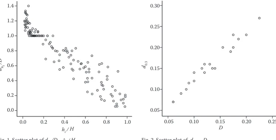
[image:4.595.66.533.73.251.2]

Figs. 1 and 2 show that linear regression is ap-propriate for both sample size methods. In the first case of sample size estimation, from the applica-tion of simple linear regression to the pre-sample data of 136 observations with the dependent vari-able being the relative diameter d_hi/D where d_hi is the diameter at height h_i and D the breast height diameter, and the independent variable being the relative height hi /H where H is the total height, resulted the equation:

Table 1. Summary statistics for the two samples

Statistics dhj

D

h_i

H d0.3 (m) D (m)

Mean 0.762 0.382 0.158 0.131

Standard error 0.030 0.027 0.012 0.011

Median 0.833 0.294 0.150 0.125

Variance 0.124 0.097 0.003 0.002

Kurtosis –0.937 –1.207 –0.594 –0.736

Skewness –0.431 0.462 0.201 0.263

Range 1.347 0.965 0.200 0.165

Minimum 0.053 0.018 0.070 0.060

Maximum 1.400 0.983 0.270 0.225

Number of values 136 136 20 20

1.4

1.2

1.0

0.8

0.6

0.4

0.2

0.0 dh i

/D

0.0 0.2 0.4 0.6 0.8 1.0

h_i / H

0.30

0.25

0.20

0.15

0.10

0.05 d0.3

0.05 0.10 0.15 0.20 0.25

D

[image:4.595.68.530.513.748.2]

d_{hi hi}

––– = 1.171 – 1.073 –––

D H

The equation was fitted to the data and resulted in a standard error of estimated values σˆ = 0.1123 and an adjusted coefficient of determination R2 _{= 0.898.} Hypothesis tests for the regression coefficients re-sulted in large values of t (76.726 and –34.572 for the constant term and the coefficient of the independent variable, respectively), which results in significance of values less than 0.05 (0.0000 for both coefficients). Consequently, the two coefficients differ from zero (P < 0.05). The value of F from the analysis of variance was F = 1,195.239 (P < 0.01).

The acceptable error, which was predefined, was equal to 10% of the independent variable mean, that is:

W_i = 0.10X– = 0.10 × 0.3817 = 0.03817

The most demanding value of the independent variable, as for the sample size, is X_i = 0.9826, which requires a sample size of 825 observations.

In the second case of sample size estimation, from the application of simple linear regression to the pre-sample data of 20 trees with the dependent variable being the diameter at stump height d_0.3 and the in-dependent variable being the breast height diameter

D, the following equation was obtained:

d_0.3 = 1.202D

Regression analysis without a constant term was used because regression analysis with constant term resulted in a constant term value not different from zero (P > 0.05).

The equation was fitted to the data and resulted in a standard error of estimated values σˆ = 0.0111 and an adjusted coefficient of determination R2 _{= 0.996.} Hypothesis tests for the regression coefficient result-ed in a large value of t (66.856), which corresponds to

P < 0.05. The value of F from the analysis of variance was F = 4,469.734, which corresponds to P < 0.01.

The acceptable error, which was predefined, was equal to 10% of the independent variable mean, that is:

W_i = 0.10X– = 0.10 × 0.1308 = 0.01308

The most demanding value of the independent variable with respect to the sample size is X_i = 0.2250, which requires a sample size of 77 observations, that is 77 trees.

Basic regression hypothesis

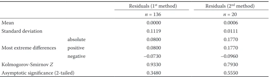
Looking at Table 2, we see that for a 5% probabil-ity the residuals for both regressions approach the normal distribution (sigΖ = 0.348 > 0.05 and sigΖ =

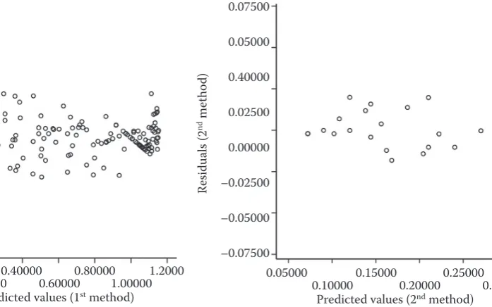
= 0.555 > 0.05). Also, the means of the residuals for both regressions are close to zero (Table 2). The sig-nificance of L is greater than the probability α = 0.05 in the homogeneity of variance test; hence the re-siduals have homogeneous variance (Table 3). Figs. 3 and 4 show that the variances of residuals for both regressions are constant (the points of the graphics assemble in a thin horizontal strip around zero, with no obvious pattern).

CoNCluSIoNS

[image:5.595.64.539.619.753.2]

For the estimation of a minimum required sample size for acceptable error of 10% of the independent variable mean, simple linear regression analysis was applied to data from a pre-sample of 20 trees. In the first case, the pre-sample had a total of 136 observa-tions, which is the number of observed diameters in all 20 trees. The relative heights were used as the independent variable and the relative diameters as the dependent variable. The estimated minimum re-quired size of the final sample calculated was 825 ob-servations (825 diameters). In the second case, the

Table 2. Kolmogorov-Smirnov normality test

Residuals (1st _{method) Residuals (2}nd _method)

n = 136 n = 20

Mean 0.0000 0.0006

Standard deviation 0.1119 0.0111

Most extreme differences

absolute 0.0800 0.1770

positive 0.0800 0.1770

negative –0.0730 –0.0960

Kolmogorov-Smirnov Z 0.9330 0.7930

pre-sample had a total of 20 observations. The breast height diameters were used as the independent vari-able and the diameters at stump height as the depend-ent variable. The minimum required size of the final sample calculated was 77 observations (77 trees). In both cases, the regression residuals were normally distributed, with constant variance and zero mean, so both methods are efficient from the validity stand-point. If we want to take into account both the cost of sampling and the precision, we must prefer the first case of a target number of individual diameters to observe, since we can measure a given number of di-ameters on any number of individual trees (less than the 77 trees that we found in the second case).

References

AVERy T., 1975. Natural Resources Measurements. 2nd _Ed.

New york, McGraw Hill Book Co.: 428.

BEHRE C., 1923. Preliminary notes on studies of tree form. Journal of Forestry, 21: 507–511.

BEHRE C., 1927. Form-class Taper curves and volume tables and their application. Journal of Agricultural Research, 35: 673–744.

BuRKHART H., GREGOIRE T., 1994. Forest Biometrics. In: PATIL G., RAO C. (eds), Environmental Statistics (Handbook of Statistics). Amsterdam, Elsevier Science: 377–407.

CHAKRAVARTI I., LAHA R., ROy J., 1967. Handbook of Methods of Applied Statistics. Volume I. London, John Wiley and Sons, Inc.

CORMIER K., REICH R., CzAPLEWSKI R., BECHTOLD W., 1992. Evaluation of weighted regression and sample size developing a taper model for loblolly pine. Forest Ecology and Management, 53: 65–76.

CORONA P., FERRARA A., 1990. Growth measuring tech-niques in forest assessment. Global Natural Resource Monitoring and Assessments: Preparing for the 21st

cen-tury. In: Proceedings of the International Conference and Workshop, 3: 1130–1132.

CORONA P., FERRARA A., 1991. Measuring techniques for assessing basal area increment of forest stands. Forest inventories in Europe with special reference to statistical methods. In: Proceedings of IuFRO Conference at Bir-mensdorf, Switzerland: 70–81.

DEMAERSCHALK J., KOzAK A., 1974. Suggestions and criteria for more effective regression sampling. Canadian Journal of Forest Research, 4: 341–348.

DEMAERSCHALK J., KOzAK A., 1975. Suggestions and criteria for more effective regression sampling 2. Canadian Journal of Forest Research, 5: 496–497.

DRAPER N., SMITH H., 1997. Applied Regression Analysis. New york, John Wiley and Sons, Inc.: 835.

ELFuING G., 1952. Optimum allocation in linear regression theory. Annals of Mathematical Statistics, 23: 255–262. ELSIDDIG E., HETHERINGTON J., 1982. The stem and

branch volume of Acacia nicotica in the fung region in Su-Table 3. Levene’s homogeneity of variance test

Levene’s

statistic L Significance

1st _{sample 0.205 0.652}

2nd _{sample 1.509 0.235}

0.80000

0.60000

0.40000

0.20000

0.00000

–0.20000

–0.40000

–0.60000

Re

sidu

al

s (1

st me

tho

d)

0.00000 0.40000 0.80000 1.2000 0.20000 0.60000 1.00000

Predicted values (1st _method)

0.07500

0.05000

0.40000

0.02500

0.00000

–0.02500

–0.05000

–0.07500

Re

sidu

al

s (2

nd me

tho

d)

0.05000 0.15000 0.25000 0.10000 0.20000 0.30000

Predicted values (2nd _method)

Fig. 3. Scatter plot for testing homogeneity of variance (1st _{regression line)}

[image:6.595.165.514.53.271.2] [image:6.595.66.339.56.272.2] [image:6.595.63.290.349.405.2]

dan. Bangor N. Wales, university College of North Wales, Department of Forestry and Wood Science: 54.

FREESE F., 1956. Guidebook for Statistical Transients. uSDA Forest Service, South Forest Experimental Station: 77. FREESE F., 1962. Elementary Forest Sampling. uSDA Forest

Service, Agricultural Handbook No. 232: 91.

GOuLDING C., MuRRAy J., 1975. Polynomial taper equa-tions that are compatible with tree volume equaequa-tions. New zealand Journal of Forest Science, 5: 313–322.

GRAy H., 1956. The form and taper of forest tree stems. Ox-ford Imperial Forestry Institute, Paper No. 32: 79.

HOEL P., 1958. Efficiency problems in polynomial estimation. Annals of Mathematical Statistics, 29: 1134–1150. HOJER A., 1903. Growth of Scots pine and Norway spruce.

Stockholm, Bilaga till. Loven, F.A. om vara barrskorar. KITIKIDOu K., 2002. A study of the form of Hungarian

oak trees (Quercus conferta) at Cholomonda Chalkidiki, Northern Greece. [Ph.D. Thesis.] Aristotelian university of Thessaloniki, Greece: 247. (In Greek)

KITIKIDOu K., 2005. Applied statistics with use of the SPSS statistical package. Thessaloniki, Tziola Publications: 288. (In Greek)

KOzAK A., SMITH J., 1993. Standards for evaluating taper estimating systems. The Forestry Chronicle, 69: 438–444. LAyLOCK P., 1972. Convex loss applied to design in

regres-sion problems. Journal of the Royal Statistical Association,

34: 148–186.

MARSHALL P., DEMAERSCHALK J., 1986. A strategy for efficient sample selection in simple linear regression

prob-lems with unequal per unit sampling costs. The Forestry Chronicle, 62: 16–19.

MAx T., BuRKHART H., 1976. Segmented polynomial regression applied to taper equations. Forest Science, 22: 283–289.

NETER J., WASSERMAN W., 1974. Applied Linear Sta-tistical Models. Regression, Analysis of Variance and Experimental Designs. 3rd _{Ed. Boston, Richard D. Irwin,}

Inc.: 1184.

NETER J., WASSERMAN W., KuTNER M., 1990. Applied Linear Statistical Models. 3rd _{Ed. Homewood, Richard D.}

Irwin, Inc.: 1181.

NORuSIS M., 2002. SPSS 11.0 Guide to Data Analysis. Chi-cago, Prentice Hall: 637.

PEREz D., BuRKHART H., STIFF C., 1990. A variable-form taper function for Pinus oocarpa Schiede in central Hon-duras. Forest Science, 36: 186–191.

PHILIP M., 1994. Measuring Trees and Forests. London,CAB International: 310.

SINGH B., SEDRANSK J., 1978. Sample size selection in regression analysis when there is nonresponse. Journal of the American Statistical Association, 73: 362–365. WyNN H., 1972. Results in the theory and construction of

D-optimum experimental designs. Journal of the Royal Statistical Society, 34: 133–147.

Received for publication October 12, 2007 Accepted after corrections February 12, 2008

Corresponding author:

Kitikidou Kyriaki, Ph.D., Dimokritos university of Thrace, Department of Forestry and Management of the Environment and Natural Resources, Laboratory of Forest Biometry, Anixis 14, Thessaloniki 54352, Greece tel.: + 30 2310 914 743, e-mail: [email protected]

odhad vhodné velikosti vzorku ke stanovení tvarových křivek kmene

aBStRaKt: Mnoho prací se zabývá hledáním vhodných tvarových křivek kmene, ale zatím bylo věnováno málo pozornosti otázce, jak velký vzorek měřených kmenů je k řešení této otázky dostatečný. V příspěvku je k nalezení vhodných rovnic použita metoda, vyžadující dvě proměnné, které jsou vzájemně lineárně korelovány. Testovány jsou potom dva soubory dat o různé velikosti. V prvním případě je velikost potřebného souboru dat vztažena k počtu průměrů měřených na jednotlivých kmenech. Ve druhém případě je velikost souboru vztažena k počtu kmenů. Analýza ukázala, že obě metody jsou vhodné z hlediska statistického hodnocení, ale první metoda je ekonomicky výhodnější. Je totiž snazší a levnější měřit další průměr na zvoleném kmeni, než měřit další kmen.