Methods of variance component estimation

INTRODUCTION

We describe methods of variance component esti-mation for the simplest case, the one-way ANOVA, and demonstrate most of them by some data sets. For this purpose we assume that a sample of a levels

of a random factor A has been drawn from the

uni-verse of factor levels which is assumed to be large. Not to be too abstract let us assume that the levels

are sires. From the i-th sire a random sample of n_i

daughters is drawn and their milk yield y_ij recorded.

The scheme of the _a

N = Σ n_i i=1

observations is given in Table 1. This case is called balanced if for each of the sires the same number of daughters has been selected. Balancedness in higher nested classification means equal subclass numbers as well as equal numbers of levels of nest-ed factors within each of the levels of factors of a higher order in the hierarchy. Some of the methods described below differ from others only in the case of unbalanced data, which means in the one-way ANOVA that not for all the sires the number of daughters is the same. Therefore we simulated an unbalanced data set.

Not for all methods formulae will be given and only the principle is explained. The reason is that we wrote this paper mainly for non-mathematicians who often use several methods and need some basic understanding of what they are doing in applying special methods. Advantages and disadvantages of the methods are discussed.

According to Rasch et al. (1999) the model equa-tion is given in (1)

y_ij= E(y_ij) + e_ij = µ + a_i + e_ij

i = 1, …, a; j = 1, …, n_i (1)

where: ai = the main effects of the levels Ai. They are

random variables eij = the errors, also random µ = constant = the overall mean

Model (1) is completed by the assumptions (E() = expectation of = mean of; V() = variance of) E(a_i) = 0, V(a_i) = σ2

a , E(eij) = 0, V(eij) = σ2; all

com-ponents on the right side of (1) are independent (2)

σ and σ2 _{are called variance components.}

The total number of observations is always denot-ed by N, in the balancdenot-ed case we have N = an. In the sequel we give the formulae for the balanced case, generalization can be found in the references.

Let us assume that all the random variables in (1) are normally distributed even if this is not needed for all the methods.

Methods of variance component estimation

D. Rasch, O. Mašata

Biometric Unit, Research Institute of Animal Production, Prague-Uhříněves, Czech Republic

ABSTRACT: Estimation of variance components is a method often used in population genetics and applied in animal breeding. Even experienced population geneticists nowadays feel lost if confronted with the huge set of different methods of variance component estimation. Especially because there exists no uniformly best method, a decision which method should be used is often difficult to take. This paper gives a complete overview of methods existing in the simplest case of a one-way lay-out and demonstrates some of them by a numerical example for which the true situation is known. Of course, the one-way lay-out is of limited practical interest but can best be used to explain animal scientists the basic principles of the methods. These basic principles are principally also valid for higher classifications. Advantages and disadvantages of the methods are discussed. The symbols used are the standard biometric symbols as given in Rasch et al. (1994). We can say that all the methods offered by SPSS can be recommended.

The normal distribution (Gauss-distribution) has the density (or likelihood) function

1 1

f(y) = e (y – µ)2 (σ >0) (3) σ√2π

2σ2

We say that y is N(µ; σ2_{)-distributed. If we have a}

random sample yT _{= (y}

i, ....,yn), its density is equal

to the product of the densities of its components. From (1), (2) and the normality assumption it

follows that the a_i and the e_ij are independently of

each other N(0;σ_a2 _{)- and N(0;σ}2_{)-distributed,}

re-spectively. The y_ij are not independently of each

other N(µ; σ2_{+ σ}

a2 )-distributed. The dependence

exists between variables within the same factor level because

cov(y_ij, y_il) = cov(µ + a_i + e_ij, µ + a_i + e_il) = = cov(a_i, a_i) = var(a_i) = σ_a2 _{if j ≠ 1}

A standardized measure of this dependence is the intra-class correlation coefficient

σ _a2

ρ_IC = (4)

σa2 + σ2

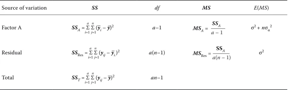
The analysis of variance (ANOVA) table is that of Table 2.

In Table 2 and the sequel we use standard nota-tion with SS = sum of squares, MS = mean squares, df = degrees of freedom, res = residual, T = total and E() = expectation of. Further a dot in place of a suffix means summation over that suffix and an additional bar above the y means dividing by the number of summands. Especially we have

1 ni

y_i. = Σ y_ij ni j=1

The column “expected mean squares – E(MS)” in Table 2 is helpful to evaluate variance component estimators by the ANOVA method.

Some of the methods are developed for unbal-anced data. Therefore we also assume a generaliza-tion of (1) by a general linear model for one random factor in (5).

Y = Xα + Uβ + e (5)

with random vectors Y and e of length N, design

matrices X (Nxq) and U (Nxm), vector α of length q with fixed effects and random vector β of length m. We complete the model (5) by the following assumptions:

rank(X) = q; rank(U) = m.

The vectors e and β are independently normally distributed with expectation vector zero and

cov-ariance matrix σ2_I

N and σa2 Im, respectively.

For more details and application in genetics see Sorensen and Gianola (2002).

The numerical example

By random number generation we received a data

set with a = 100 sires with n_i daughters as given

in Table 3. We had in mind milk yields of heifers during the full first lactation with an assumed herit-ability coefficient.

Table 1. Observations in a one-way layout of ANOVA – unbalanced case

Level A₁ Level A₂ … Level A_a

y₁₁ y₂₁ … y_a1

y₁₂ y₂₂ . y_a2

. . . .

. . .

y1n₁ y2n₂ … y_ana

Table 2. ANOVA table of one-way ANOVA model II in the balanced case

Source of variation SS df MS E(MS)

Factor A

_{a n}

SS_A = Σ Σ (y_i – y)2

i=1 j=1

a–1 _MS SSA A =

a – 1 σ

2 _{+ nσ} α2

Residual

_{a n}

SS_Res = Σ Σ (y_ij – y_i.)2

i=1 j=1

a(n–1) _MS SSA

Res =

a(n – 1) σ

2

Total

_{a n}

SS_T = Σ Σ (y_ij – y)2

i=1 j=1

σ2 g

h2 _{= = 0.4}

σ2g + σ2

Because 1 σ2

α = σ2g ,

4

this can be verified for instance by σ2 _{= 6 and σ}2

α = 1.

Without loss of generality the overall mean was put equal to µ = 7 000. By (4) we get

1_ρ

IC = = 0.14283

1 + 6

The data were generated in two steps. For both steps we used the pseudo-random-number genera-tor of SPSS (transform – compute), which generates normally distributed random numbers with given

mean and variance. At first we generated the 100 sire means distributed as N(7 000, 1). The

num-bers were repeated n_i times for each of the sires

according to Table 3. In the second step to all of these values we added the effect of random error (environmental effect) distributed as N(0, 6). In this way we got a simulated value for each daughter.

In Figure 1 a part of the data is shown. The number of the sires can be found in the first column.

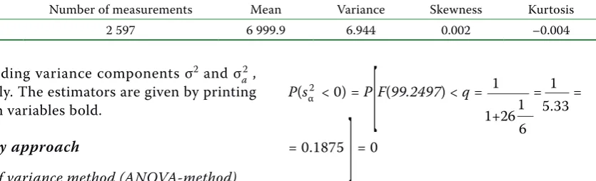
In Figure 2 the SPSS output of simple descriptive statistics over all data is shown.

Figure 2 shows that our random number genera-tor works well. Mean (7 000) and total variance (7) is represented quite well and normality is reached because the estimated values of skewness and kur-tosis are negligible (these parameters are zero in normal distributions). We therefore can use our

Table 3. Numbers of daughters of 100 sires

Sire 1–30 n_i = 30 Sire 71–75 n_i = 23

Sire 31–41 ni = 29 Sire 76–80 ni = 22

Sire 42–50 n_i = 28 Sire 81–85 n_i = 21

Sire 51–56 n_i = 27 Sire 86–90 n_i = 20

Sire 57–60 ni = 26 Sire 91–95 ni = 19

Sire 61–65 n_i = 25 Sire 96–100 n_i = 18

Sire 66–70 ni = 24

generated data set to compare the different meth-ods of variance component estimation for the

one-way-ANOVA. Methods giving estimates near σ2

a = 1

and σ2 _{= 6 as used in the data generation are}

ac-ceptable.

Properties of estimators

Before we discuss the different methods of esti-mating the variance components, we will introduce some theory about estimators. The following ran-dom variables can also be vectors – it follows from the context when this is the case.

Definition 1: The estimator θˆ = θˆ (y) is a

map-ping of a random sample y = (y₁,…, y_n)T _{(T means a}

transposed vector) of size n on the parameter space of parameter θ of the distribution of this sample. The realization of the estimator is called an esti-mate θˆ (y).

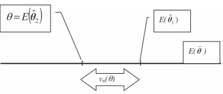
Definition 2: The estimator θˆ = θˆ (y) is unbiased if Eθˆ = θ. The difference E(θˆ ) – θ = v_n(θ) is the bias of the estimator. The bias of an unbiased estimator is zero. The expression

E[{θˆ – θ}2_{] = V(θˆ ) + v}2 n (θ)

is called the mean squared error of θˆ = θˆ (y) (MSE). The mean squared error of an unbiased estimator equals its variance.

In Figure 2 θˆ ₁ is biased and θˆ ₂ is unbiased. Example 1: The estimator

_n

Σ yi i=1 µˆ = = y–

n

of the mean µ of the components of a random sam-ple y_T = (y₁, ..., y_n) is unbiased.

Definition 3: The estimator θˆ = θˆ (y) of θ is called minimum variance (or best) unbiased lin-ear (MVUL) or quadratic (MVUQ) estimator if its variance is minimum amongst all unbiased linear and quadratic estimators, respectively.

Definition 4: The estimator θˆ = θˆ (y) of θ is called minimum mean squared error estimator (MMSE) if its mean squared error MSE is minimum.

The estimator _n

Σ yi i=1 µˆ = = y–

m

of the mean µ in example 1 is a minimum vari-ance (or best) unbiased linear estimator, shortly a BLUE.

Definition 5: Let f(y, θ) be the density function of θ, the parameter of the distribution of a random variable y. This is a function of two variables, θ and y. If we call it density function, we consider it as a function of y for fixed θ. But the same function f(y, θ) as a function of θ for fixed y is called likelihood function. If we estimate θ so that it will maximize the likelihood function in the parameter space of θ, we call the corresponding estimator Maximum-Likelihood Estimator (MLE).

Definition 6: The estimator is called minimum norm quadratic unbiased invariant estimator – MINQUE, if it is a quadratic form of Y in (5), unbiased and in-variant against the translation of fixed effect Xα in (5) and minimizing a matrix norm. For more details see Rao (1971), the first paper on MINQUE.

Before we discuss some of the existing methods of estimation, let us make a general remark. In (1) the model equation of the random variables y is given. Its realisations as well as the data observed are de-noted by the non-bold letter y. Mathematical opera-tions as minimizing (least squares) or maximizing (likelihood) can be performed for the realizations only. The result of such an optimisation is the es-timate, the function of the y. If this is an explicit formula, we obtain the estimator by replacing the y-s in that formula by the random variables y. In implicit formulae the estimator cannot be repre-sented in closed form but nevertheless some (often asymptotic) properties can be derived.

Estimation of the variance components

We first present methods for the so-called fre-quency approach. In this approach we assume that the parameters of the distribution and by this especially the overall mean and the variance components are fixed but unknown real values or vectors. In the sequel we use for all the methods

the same symbols s2 _{and s}

α2 for the estimates of the

2

ˆ

ș

E

T

vn(T)

E(ș)

corresponding variance components σ2 _{and σ} a2 ,

respectively. The estimators are given by printing all random variables bold.

Frequency approach

Analysis of variance method (ANOVA-method) The oldest and simplest method of estimating the two variance components is due to Fisher (1925). In this method we replace in the column E(MS) of the ANOVA table the variance components any σ by its estimate s and put the resulting expressions equal to the observed MS and finally we solve the resulting equations. In our special case of the bal-anced one-way classification this leads to

s2 _{+ ns}

α2 = MSA

s2 _{= MS}

res

Solving these equations gives:

s2 _{= MS}

res (6)

1 s_α2 _{= (MS}

A – MSres ) (7)

n

Properties of the estimators

Minimum variance unbiased quadratic estima-tor for any continuous distribution with existing first two moments (milk yield, body weight and so on) and Minimum variance quadratic estima-tor for normal distributions. These are not always estimators because (7) can become negative, which means that it is not a mapping into the parameter space (the positive real line) as necessary for the estimator according to definition 1. The probability of a negative estimator is given by

1 P(s_α2 _{< 0) = P}

[

]

In (8) F(a– 1, a(n – 1)) is a random variable with an F–distribution with a–1 and a(n–1) d.f. Tables for these probabilities are given by Verdooren (1982).

If in our simulated example we assume ap-proximately a mean sample size of 26, formula (8) gives

1 1 P(s_α2 _{< 0) = P}

[

1 =

= 0.1875

]

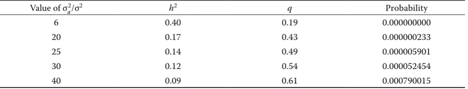
For some other values of σ_a2 _{and σ}2 _the

corre-sponding probabilities can be found in Table 4. To have a real chance to find negative estimates, the environmental variance should be for instan-ce 30 instead of 6 or the degrees of freedom must be smaller (this means, we expect negative esti-mates only for insufficient sample sizes). Therefore negative estimates should not be expected in our simulation study.

Quasi-maximum-likelihood method (QML) A maximum likelihood estimate is obtained by minimizing the likelihood function of the sample under the restriction that the solution lies in the parameter space. Without this restriction some variance components may be negative. Because we then do not have an estimator in the sense of definition 1, we call the method quasi-maximum-likelihood method. If we replace in this minimum the realizations of the random variables by the random variables, we obtain the quasi-maximum likelihood estimator. Because the family of nor-mal distributions is a two-parametric exponential family with the set of complete minimal sufficient statistics (see Rasch, 1995)

1 a n

y.. = Σ Σy_ij, SS_res, SS_A ani=1 j=1

the likelihood function of the data in Table 1 can be written as

1 1 1 1

_e

{

[

]}

f(y₁₁, ..., y_ab) = (2π)an(σ2₎a(n – 1)_(σ2 _+σ2

a ) a

2 2 2

Deriving the logarithm2 _{of this likelihood}

func-tion with respect to µ and the two variance com-ponents without side conditions to restrict the solutions to the parameter space leads to the fol-lowing estimators:

Table 4. Descriptive statistics of 2 597 milk yields

Character Number of measurements Mean Variance Skewness Kurtosis

µˆ = -y s2 _{= MS}

res (9)

1 a – 1 s_α2 _{= ( MS}

A – MSres) (10)

n a

Equations (6) and (9) are identical, s_α2 _{in (10) is}

biased and has a higher probability of becoming negative than the estimator in (7). The estimator of µ is needed to replace the µ in the equations stemming from the derivations with respect to the variance components only.

Maximum-likelihood method (ML)

Herbach (1959) derived a real maximum likeli-hood estimator (solutions restricted to the param-eter space).

SS_res + SS_A

s2 _{= min}

[

res,

]

an 1 a – 1 s2

a = max

{[

]

}

n a

Both estimators are biased.

Restricted maximum-likelihood method (REML) Anderson and Bancroft (1952) introduced a re-stricted ML method. This method uses a translation invariant restricted likelihood function depending on the variance components to be estimated only and not on the fixed effects like µ. This restricted likelihood function as a function of the sufficient statistics for the variance components. The latter is then derived with respect to the variance com-ponents under the restriction that the solutions are non-negative. The solutions are:

SS_res + SS_A

s2 _{= min[MS}

res, ] (13)

an– 1

1 s2

a = max

{[

]

}

n

Modified maximum-likelihood method (MML) Stein (1964) and Kotz et al. (1969) found modified ML-estimators which have uniformly smaller mean squared error compared with the ML estimators of Herbach in (11) and (12). They are given by:

SS_res + SS_A SS_res + SS_A + any– 2

s2 _{= min[MS}

res, , ] (15)

an + 1 an + 2 1 a – 1

s2

a = min

〈

{[

]

}

n a + 1 SS_A + any– 2

{[

]

}

〉

an + 2 Federer’s estimator

From the Bayesian aspect it could be shown that some of the truncated estimators above are inadmissible. The following non-truncated and nonnegative estimators could not be proved to be inadmissible but they were not proved to be admis-sible either (there is no uniformly better estima-tor). The advantage of the estimators proposed by Federer (1968) is that they and their distribution function can be expressed in an analytical form.

s2 _{= MS}

res (17)

1 s_a2 _{= [MS}

A – MSres (1 – e–δMSA)] (18)

n

For δ Federer proposed to choose a value in the interval

1 δ ∈

[

]

Minimum-norm and minimum-variance quadratic unbiased estimators (MINQUE)

We now consider model equation (5) with its side conditions. This model is especially useful if we consider higher classifications and mixed models. In this case the estimator is called invariant if it is

Table 5. Probabilities of negative estimates for f₁ = 99, f₂ = 2 497, n = 26 and severalvalues of σ_a2

Value of σ_a2 _/σ2 _h2 _{q Probability}

6 0.40 0.19 0.000000000

20 0.17 0.43 0.000000233

25 0.14 0.49 0.000005901

30 0.12 0.54 0.000052454

not influenced by the translation of non-random elements of the model. Rao (1971a, 1972) devel-oped methods to estimate linear combinations of all the variance components in model (5). We will not go into details because for an understanding some knowledge of matrix algebra is needed. The basic idea is to find unbiased quadratic estimators which are invariant and minimize some matrix norm. Unfortunately, the solution in the most in-teresting cases depends on the unknown variance components. If they are replaced by estimates from the data, the solution is neither unbiased nor quad-ratic any longer. In SPSS the MINQUE procedure is the default method. MINQUE can result in negative estimates and the method to avoid this leads to neither unbiased nor quadratic estimators again. Minimum-variance and minimum-mean squared error quadratic estimator

These procedures were developed mainly by Rao (1971b) and LaMotte (1973). The basic idea is to

determine the matrix A of a quadratic form YT _AY

of the vector Y in (5) so that an unbiased estimator with minimum variance (Rao, 1971b) or an estima-tor with minimum mean squared error (LaMotte, 1973) is obtained. On principle, the same problems arise as with the MINQUE procedure.

There are further proposals for estimators but we consider those discussed above as the most im-portant ones from the practical point of view. For more details and variation of the above methods see Sarhai and Ojeda (2004, 2005).

Bayesian and empirical Bayesian approach and Markov chain Monte Carlo (MCMC) methods

We now only shortly mention methods for the so-called Bayesian approach. In this approach we assume that the parameters of the distribution and by this especially the variance components are ran-dom variables with some prior knowledge of their distribution. This prior knowledge is sometimes given by an a priori distribution, sometimes by data from an earlier experiment. This prior distribution is combined with the likelihood of the sample re-sulting in a posterior distribution. The estimator is used in such a way that it minimizes the so-called Bayes risk. If we use the squared error loss as this risk, the mean of the marginal posterior distribu-tion is the Bayes estimator. The problem is the selection of a posterior distribution which should

cover the user’s knowledge (or imagination) of the unknown parameters to be estimated. So-called non-informative prior distribution is often used which in the one-way lay-out leads exactly to the Quasi-Maximum-Likehood method (QML). For more details see Gelman et al. (1995).

Method of Tiao and Tan

We explain the Bayes method by an approach of Tiao and Tan (1965). We assume like in (QML) that the random variables on the left side in (1) are normally distributed with the likelihood function given in QML

1 1 1 1

_e

{

[

]}

f(y₁₁, ..., y_ab) = (2π)an(σ2₎a(n – 1)_(σ2 _+σ2

a ) a

2 ₂ 2

For the three parameters µ, σ2_{, σ}2

a the prior

dis-tribution is chosen as: 1

f_prior( ), 0 < σ2 _{< σ}2 _{+ σ}2

a (19)

σ2 (σ2 + σ2a )

By combining the prior with the likelihood function gives the posterior distribution proportional to

f_posterior(µ, σ2_{, σ}2

a |y11, ..., yab) ∝

1 1 1 1

_e

{

[

]}

∝ (2π)an(σ2₎a(n – 1)_(σ2 _+σ2

a ) a

2

2 2

Integrating over µ yields in the marginal distribu-tion of the two variance components.

We now obtain the marginal distribution of each of the variance components by integrating over the other one. This leads to integral equations which can be solved by some computer programs.

For a squared error loss as the Bayes risk Klotz et al. (1969) found the Bayes estimators.

Gibbs sampling

Gibbs sampling is mainly used in the Bayesian context. Shortly spoken it is an iterative improve-ment of prior information.

Before we discuss the Gibbs sampling, we will define what is understood by data augmentation.

Let a posterior density be given by p(θ|y) =

∫

z

p(z|y) = denotes the predictive density of some so-called latent data z

p(θ|y,z) = the conditional density of θ given the so-called augmented data x = (y,z)

Then the predictive density is given by p(z|y) =

∫

z

where: p(z|φ,y) = the conditional predictive density

After substitution and interchanging the order of integration we obtain

g(θ) =

∫

K(θ,φ) =

∫

and

g(θ) = p(θ|y)

Starting with some initial

g₀(θ) we solve (22) by iteration via

g_i+1(θ) =

∫

Gibbs sampling is based on so-called chained data augmentation (the chain is a Markov chain and Gibbs sampling is a multivariate special type of MCMC = Markov chain Monte Carlo).

When the (considered as a random variable) unknown parameter is a vector – as it is usually the case in variance component estimation – then the procedure works as follows. At first we have to know or to assume the conditional densities of each of the components of

θT _{= (θ}

1, ..., θp)

given the other components. We start with some

initial value θT

0 = (θ10 , ..., θp0 ) of θT = (θ1, ..., θp) and

then iterate where each iteration is defined by the following loop:

Sample θ₁i +1 _{from p(θ}

1|θ2i , ... , θ , y);pi

Sample θ₂i +1 _{from p(θ}

2|θ1i +1, θ , ..., θ3i p , y);i

. .

Sample θ_pi +1 _{from p(θ}

p|θ1i +1, ..., θpi –+ 11 , y)

As a good tool for those who want to be deeply engaged in Gibbs sampling we recommend two Fortran programs described in Reinsch (1996) and for the theoretical background to Gamerman (1997).

Results of some methods of variance component estimation

Results of the methods ANOVA, QML, REML and MINQUE could be obtained via the SPSS menu

Analyze

General linear model

Variance components

and then selecting the methods by the button “op-tions”.

Federer’s method was not used because it assumes balanced data which need not really occur in animal breeding. MIVQUE was calculated by SAS.

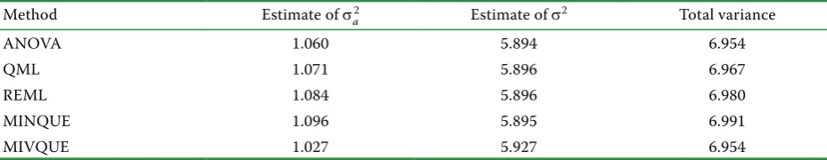
The results of the methods applied to our gener-ated data set are shown in Table 6.

The methods differ only slightly from each other. By all methods the variance component between the sires is a little bit overestimated while the re-sidual variance component is a bit underestimated. The total variance (known to be 7) is estimated quite well by all methods. And all methods seem to work quite well in unbalanced one-way ANOVA models. But this may be quite different for higher classifications and covariates in the models.

Such conclusions can be drawn only if we apply the different methods to a data set for which the parameters are known like in our simulated data. Otherwise we can only see differences between the methods but we do not know which of them is good.

Table 6. Estimates of the variance components from the data set by different methods

Method Estimate of σ_a2 _{Estimate of σ}2 _{Total variance}

ANOVA 1.060 5.894 6.954

QML 1.071 5.896 6.967

REML 1.084 5.896 6.980

MINQUE 1.096 5.895 6.991

REFERENCES

Anderson R.L., Bancroft T.A. (1952): Statistical Theory in Research. McGraw-Hill, New York.

Federer W.T. (1968): Non-negative estimators for com-ponents of variance. Appl. Stat., 17, 171–174.

Fisher R.A. (1925): Statistical Methods for Research Workers, Oliver and Boyd.

Gamerman D. (1997): Markov Chain Monte Carlo. Chap-man and Hall, New York.

Gelman A., Carlin J.B., Stern H.S., Rubin D.B. (1995): Bayesian Data Analysis. Chapman and Hall, New York.

Herbach L.H. (1959): Properties of model II type analy-sis of variance tests A: Optimum nature of the F-test for model II in balanced case. Ann. Math. Statist., 30, 939–959.

Klotz J.H., Milton R.C., Zacks S. (1969): Mean square efficiency of estimators of variance components. J. Am. Stat. Assoc., 64, 1383–1402.

LaMotte L.R. (1973): Quadratic estimation of variance components. Biometrics, 29, 311–330.

Rao C.R. (1971a): Estimation of variance and covariance components: MINQUE theory. J. Multivar. Anal., 1, 257–275.

Rao C.R. (1971b): Minimum variance quadratic unbiased estimation of variance components. J. Multivar. Anal.,

1, 445–456.

Rao C.R. (1972): Estimation of variance and covariance components in linear models. J. Am. Stat. Assoc., 67, 112–115.

Rasch D. (1995): Mathematische Statistik. Joh. Ambrosius Barth and Wiley, Berlin, Heidelberg. 851 p.

Rasch D., Tiku M.L., Sumpf D. (1994): Elsevier’s Diction-ary of Biometry. Elsevier, Amsterdam, London, New York.

Rasch D., Verdooren L.R., Gowers J.I. (1999): Fundamen-tals in the Design and Analysis of Experiments and Surveys – Grundlagen der Planung und Auswertung von Versuchen und Erhebungen. Oldenbourg Verlag, München, Wien.

Reinsch N. (1996): Two Fortran programs for the Gibbs Sampler in univariate linear mixed models. Dummer-storf. Arch. Tierz., 39, 203–209.

Sarhai H., Ojeda M.M. (2004): Analysis of Variance for Random Models, Balanced Data. Birkhäuser, Boston, Basel, Berlin.

Sarhai H., Ojeda M.M. (2005): Analysis of Variance for Random Models, Unbalanced Data. Birkhäuser, Bos-ton, Basel, Berlin.

Sorensen A., Gianola D. (2002): Likelihood, Bayesian, and MCMC Methods in Quantitative Genetics. Sprin-ger, New York.

Stein C (1969): Inadmissibility of the usual estimator for the variance of a normal distribution with unknown mean. Ann. Inst. Statist. Math. (Japan), 16, 155–160. Tiao G.C., Tan W.Y. (1965): Bayesian analysis of random

effects models in the analysis of variance I: Posterior distribution of variance components. Biometrika, 52, 37–53.

Verdooren L.R. (1982): How large is the probability for the estimate of a variance component to be negative? Biom. J., 24, 339–360.

Received: 2005–11–02 Accepted after correction: 2006–03–13

Corresponding Author

Ing. Ondřej Mašata, Biometric Unit, Research Institute of Animal Production, P.O. Box 1, 104 01 Prague-Uhříněves, Czech Republic