Partial equilibrium model – beef

(1)

Th e production of meat cattle is one of the most important branches of the livestock production. From the technological point of view, it mainly includes a full feeding of meat animals, breeding of the beef breeds of cattle (in particular the maternity population of cows without commercial production of milk) and other categories of cattle which are cast from the original, mainly dairy-oriented populations. In this respect, it includes mainly the spayed cows of the original dairy livestock, which unfortunately form a relatively high percentage of beef production and which signifi cantly worsen the economic situation for the breeders of classical meat breeds. Th e main consequence of the low purchase price of these spayed cows and their relatively high number is the enormous pressure on the low level of the purchase farmer price, which in many case moves at the level of the cost price. Meat breeds of cattle or cows without commercial production of milk (KBTPM), respectively, represent the only category of cattle not suff ering a decline in the monitored pe-riod; on the contrary, in the last decade their numbers have gradually risen. Nevertheless, generally, the long term reduction of the cattle numbers, the economic reasons, the price policy and other infl uences cause a chain of negative eff ects which subsequently show on other levels of the analyzed commodity vertical. In this respect, it includes, for example, an increase in export of the excess cattle, which, however, is

si-multaneously accompanied by the ever faster growing import of beef (but with a higher added value, because it mostly involves the already processed products), by a decrease in the consumption of feeding grain (grain fodders in general), the reduction of the consump-tion of large-volume fodders against an increase in the area of the permanent grass vegetation (TTP), by the decreased utilization of the slaughtering capacity of meat-processing companies and the related food industries or, for example, by an increasing negative balance of foreign trade. An unpleasant factor is the continuous drop in the consumption of beef. Causes for this trend can be found in various areas. For one, there has been a relatively signifi cant change in the structure of eating habits during the last 20 years. However, it is possible to point out the price develop-ment as the main cause of the decreasing consump-tion. During the observed period, beef has become the most expensive meat commodity, which is shown in the decrease of the fi nal consumer demand and its partial transfer to cheaper kinds of meat. At the same time, meat producers have reacted to the previously mentioned situation by a more frequent replacing of beef in the meat products by a cheaper equivalent. Th is has naturally led to a decrease in the amount of beef in the semi products and other products and thence its fi nal consumption has also decreased, see, e.g., Malý and Kroupová (2006).

PARTIAL EQUILIBRIUM MODEL  BEEF

Michal MALÝ

Department of Economics, Faculty of Economics and Management, Czech University of Life Sciences in Prague, Prague, Czech Republic

Abstract: Th e main goal of the presented paper is to propose, specify and quantify a model of partial equilibrium in the beef meat vertical in the Czech Republic. Characterized within the analyzed relations in the commodity vertical will be the demand-off er relationships on partial levels of the commodity chain on the basis of which the functional relations of the si-multaneous model of the above-mentioned market will subsequently be specifi ed. Th e quantifi ed model enables the defi ni-tion and descripni-tion of the main determinants of the beef off er and demand. Th e data used was acquired from the Situation and Forecast Reports (MA CZ), from the Annual Reports on the State of Agriculture (UZEI) and from the Family Accounts Statistics (CSU), for the period from 1995–2010. With regard to respecting the simultaneous relations, the model estimate was carried out by the means of the two-level method of least squares with the subsequent statistic-econometrical verifi ca-tion. Th e acquired model shows a suffi cient robustness for market analyses and the possible simulation calculations. Key words: beef, consumer, farmer, partial equilibrium model, price, producer

(2)

MATERIAL AND METHODS

The performed analysis of the beef commodity vertical was based on the principles of a commodity model of partial equilibrium (Labys and Pollak 1984), respecting three levels of the product vertical in the given market. Created at each level are the offer-de-mand relations which also further mutually intertwine among the individual subjects at different stages of the vertical, creating simultaneous bonds influenc-ing the overall concept of the model. Accordinfluenc-ing to Hallam (1990), it is possible to classify 4 basic types of commodity models based on the analytical form of the functional relations used and the manner of (non)incl uding the factor of time. The applied model of partial equilibrium can be described within the mentioned classification as linear, simultaneous and quasi-dynamic, because it includes the feed forwards and feedbacks between the explained variables with the simultaneous use of the linear functional form and the inclusion of the time vector, although without an own time differentiation of the explaining variables (delayed exogenous variables are not used).

Th e basic level of the vertical is agricultural produc-ers, who are presented in the model as subjects off er-ing livestock for the purpose of slaughter processer-ing. Th e behaviour of these farmers is determined by the prerequisite of the adaptable price expectation of the mentioned subjects (Nerlov and Bessler 2001), and from the point of functional relations, the off er of slaughter livestock is infl uenced by the total amount of full-feed cattle, by the rate of import and the farmers price of beef (TARIC classifi cation), by the amount of unit support per 1 kg of beef (for more information see the UZEI methodology) and by the time vector, see relation (1). Th e states of cattle in the full-feed category depend on the quantity of cows without commercial production of meat, on the farmer price per 1 kg of live weight as well as on the unit subsidy for 1 kg of beef, see rela-tion (2). To express the farmer price, the explaining variables included the price after processing, the time vector and the rate of import and export price of beef, see relation (3). Th e mentioned relations characterize the farm level, which is the off ering part for demand of the subsequential processing level.

Farm level:

ୗ୅ǡ୆୑ǡ୲ൌ ቆܰܥ஻ெǡ௧ǡ

ܫܲ஻ெǡ௧

ܲܣܲ஻ெǡ௧ǡ ܷܵ௧ǡ ܶቇ

(1)

Where:

Q_SA,BM,t = offered quantity of beef – production (t of live weight/year)

NC_BM,t = states of cattle (full-feed category) derived from (2), (thousand head/year)

ܰܥ஻ெǡ௧ൌ ൫ܰܯܥ஻ெǡ௧ǡ ܲܣܲ஻ெǡ௧ǡ ܷܵ௧൯ (2)

Where:

PAP_BM,t = price of agricultural producer of beef derived from (3) (CZK/kg of live weight)

ܲܣܲ஻ெǡ௧ ൌ ቆ

ܫܲ஻ெǡ௧

ܧܲ஻ெǡ௧ǡ ܲܲ஻ெǡ௧ǡ ܶቇ (3)

Where:

IP_BM,t = import price of beef (CZK/kg) EP_BM,t = export price of beef (CZK/kg)

NMC_BM,t = states of KBTPM (thousand head /year) US_t = unit subsidy (CZK/kg of liveweight/year) PP_BM,t = price after processing (CZK/kg)

T = time vector (proxy variable of technological

changes)

In the environment of the Czech Republic, the mod-elled beef market is signifi cantly determined by the foreign trade and therefore it is conceived as open in the model. Th e foreign sector can have a major infl uence on the off er side – mainly on the processing part, as well as on the demand part – mainly at the consumer level, but also at the level of processing. In accordance with a number of studies of agricultural foreign trade (e.g. the FAO summary study – Sarris and Hallam 2006), relations (4) and (5) were used for expressing the import and export of beef, whilst the import of beef is determined by the quantity of beef demanded, the price after processing and the time vector. Due to the relatively low production and long-term overhang of off er over demand, the export of beef is infl uenced only by the proportion of the export and processing price with the inclusion of the time vector.

Meat import:

ܳூெ஽ǡ஻ெǡ௧ൌ ൫ܳ஽஼஽ǡ஻ெǡ௧ǡ ܲܲ஻ெǡ௧ǡ ܶ൯ ₍₄₎

Where:

Q_IMD,BM,t = imported quantity of beef derived from (4) (thousand t of sl. weight/year)

Q_DCD,BM,t= demanded quantity of beef derived from (9) (thousand t of sl. weight/year)

PP_BM,t = price after meat processing derived from (8)

(CZK/kg)

changes)

Meat export:

ܳா௑஽ǡ஻ெǡ௧ൌ ൬ா௉_௉௉ಳಾǡ೟

ಳಾǡ೟ǡ ܶ൰

(3)

Where:

Q_EXD,BM,t = exported quantity of beef derived from (5) (thousand t of sl. weight/year)

EP_BM,t = export price of beef (CZK/kg)

(CZK/kg)

changes)

The subsequent level of the vertical represents slaughterhouses or meat processing plants, respec-tively, which include the slaughter processing of the purchased quantities of animals, when the prod-uct is first a slaughter processed body, statistically monitored under the indicator of domestic slaughter, which can be the subject of foreign trade as well as the domestic demand of the subsequent elements of the vertical. The relationship between the domestic slaughter and the processed quantity of slaughter livestock (see relation (6)) is in principle only a technological one, depending only on the slaughter yield, which is subsequently determined by, e.g., the breed, sex or age of a slaughter animal. Nevertheless, the initial processing of slaughter body is mostly accompanied by the subsequent processing and the production of chopped meat which is already a standard product of the offer at the processing plant level both for the external meat processing plants and for the end consumers. According to Hallam (1994), the amount of offer of the chopped meat is influenced by a number of exogenous and endogenous influences; for the conceived model (see relation (7)), due to the specific features of the food market in the Czech Republic, the endog-enous influences of the quantity of the imported beef meat derived from relation (4) and the price after processing were used, which according to relation (8) is determined by the price of the agricultural producer, the consumer price and the time vector. The mentioned price transmissions are based on a number of studies performed in the meat market in the Czech Republic, e.g. Lechanová (2006), and Malý (2009). The offer of meat processing plants takes into account not only the yield but also the existence of the derived meat products (meat products and semi products) which, however, are not calculated further in the conceived model.

Meat processing plant:

ܦܵ஻ெǡ௧ ൌ ൫ܳௌ஺ǡ஻ெǡ௧൯ (6)

Where:

DS_,BM,t = domestic slaughter (thous. t of slaughter weight/year)

Q_SA,BM,t = offered quantity of beef derived from relation (1) (t of live weight /year)

ܳௌ௉ǡ஻ெǡ௧ ൌ ൫ܳூெ஽ǡ஻ெǡ௧ǡ ܲܲ஻ெǡ௧൯ (7)

Where:

Q_SP,BM,t = offered quantity of chopped beef derived from (7) (thous. t/year)

Q_IMD,BM,t = imported quantity of beef derived from (4) (thous. t of sl. weight/year)

(CZK/kg)

ܲܲ஻ெǡ௧ൌ ൫ܲܣܲ஻ெǡ௧ǡ ܥܲ஻ெǡ௧ǡ ܶ൯ (8)

Where:

PAP_BM,t = price of beef agricultural producer derived from (3) (CZK/kg live weight)

CP_BM,t = consumer price of beef (CZK/kg)

changes)

Connected to the final processed meat offer, ac-cording to the classical theory of microeconomy (Varian 2002), is the partial consumer demand, which is, due to a wide range of meat products, statistically abstracted into the summary indicator of beef con-sumption. According to similarly conceived partial equilibrium models (Moro et al. 2002) and based on the microeconomy theory, the consumer demand is, according to relation (9), dependent on the consumer price of beef and on the total consumer expenses on meat expressing the amount of income which an average consumer allocates for meat consumption. Then the consumer price of beef is, according to relation (10), dependent on the processing price of beef, the consumer price of pork and chicken and on the rate of the import and export price, express-ing the motivation of a foreign sector to enter the domestic market, influencing the consumer price (Schaffer 2008).

Consumer:

ܳ஽஼஽ǡ஻ெǡ௧ൌ ൫ܥܲ஻ெǡ௧ǡ ܶܧெǡ௧൯ (9)

Where:

Q_DCD,BM,t= demanded quantity of beef derived from (9) (thous. t/year)

CP_BM,t = consumer price of beef derived from (10) (CZK/kg)

TE_M,t = total consumer expenses on meat (thous.

CZK/year)

୆୑ǡ୲ൌ ቆ୆୑ǡ୲ǡ ୔୑ǡ୲ǡ ୔୐୑ǡ୲ǡ

୆୑ǡ୲

୆୑ǡ୲ቇ

(4)

Where:

CP_BM,t = consumer price of beef (hind without bone)

(CZK/kg)

CP_PM,t = consumer price of pork (leg) (CZK/kg) CP_PLM,t = consumer price of chicken (breast) (CZK/kg) IP_BM,t = import price of beef (CZK/kg)

EP_BM,t = export price of beef (CZK/kg)

To express the equilibrium state, the model was supplemented with an umbrella balance identity.

Balance:

୍୑ୈǡ୆୑ǡ୲൅ ୗ୔ǡ୆୑ǡ୲ൌ ୈେୈǡ୆୑ǡ୲൅ ୉ଡ଼ୈǡ୆୑ǡ୲ (11)

As already mentioned above, in order to simplify the basic output of the linear function and to make estimates, the analytical form of the conceived model used was the two-level method of least squares (TSLS), which ranks among the methods with limited infor-mation, but it was applied in the Gretl 1.8.7. program environment by a one-off estimate of simultaneous equations. The compliance of the estimated equa-tions with data is standardly quantified by the means of a tested corrected coefficient of determination and the statistical verification of the estimated pa-rameters was carried out on the basis of the t-test. The subsequent econometrical presumptions were verified by the common procedures for simultaneous models (Kennedy 2008). The multicollinearity was tested using the Farrar-Glauber test (Green 2008), the autocorrelation of residuals using the Ljung-Box test (see Gujarati, 2003), the heteroskedasticity using a combined ARCH test with autocorrelation (Cipra 2008)1_{and the normality of the residual}

com-ponent using a multi-dimensional Doornik-Hansen test (Doornik and Hansen 1994).

DATA CHARACTERISTICS

The quantification of the specified commodity model of partial equilibrium in the beef market was based on the data acquired from the Situation and Forecast Reports (MZe ČR 2010), from the Annual Reports on the State of Agriculture (UZEI) and from the Family Accounts Statistics (ČSÚ), for the period from 1995–2010. Due to the character of some vari-ables which are monitored only in the time-aggregated annual values, the data base was forcibly limited by this restriction and the data of time lines was used in the estimate proper with the total number of 257 observations.

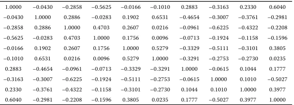
In order to verify one of the fundamental econo-metric presumptions of the non-presence of a perfect multicollinearity, a Farrar-Glauber test was performed on the base data, whilst a pair correlation matrix was quantified (Table 1). On the basis of the values of the correlation coefficients (RCC), it is obvious that the model does not contain multicollinearity of a high intensity because all RCC < 0.66.

RESULTS AND DISCUSSION

Assembled within the specification was an eleven equation simultaneous model, whose subsequent estimate was carried out by the means of the method of least squares in accordance with the principle of

[image:4.595.66.534.83.250.2]

1_{ARCH test uses the principles of the Lagrange Multiplier test (Green 2008), verifying the non-presence of a group} heteroskedasticity.

Table 1. Residual correlation matrix, C (10 × 10)

1.0000 –0.0430 –0.2858 –0.5625 –0.0166 –0.1010 0.2883 –0.3163 0.2330 0.6040 –0.0430 1.0000 0.2886 –0.0283 0.1902 0.6531 –0.4654 –0.3007 –0.3761 –0.2981 –0.2858 0.2886 1.0000 0.4703 0.2607 0.0216 –0.0961 –0.6225 –0.4322 –0.2208 –0.5625 –0.0283 0.4703 1.0000 0.1756 0.0096 –0.0713 –0.1924 –0.1158 –0.1596 –0.0166 0.1902 0.2607 0.1756 1.0000 0.5279 –0.3329 –0.5111 –0.3101 0.3805 –0.1010 0.6531 0.0216 0.0096 0.5279 1.0000 –0.3291 –0.2753 –0.2730 0.0235 0.2883 –0.4654 –0.0961 –0.0713 –0.3329 –0.3291 1.0000 –0.0615 0.1044 0.1777 –0.3163 –0.3007 –0.6225 –0.1924 –0.5111 –0.2753 –0.0615 1.0000 0.1010 –0.5027

(5)

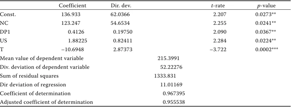
limited information. For this reason, the following interpretation pays attention gradually to the results of the quantification of the individual equations. The first explained variable in the system of equa-tions is the amount of the offer of beef at the level of the agricultural producer, whilst the estimate of the explaining variable parameters is stated in Table 2.

The outputs show that all variables have a positive effect on the amount of the offer of slaughter animals, except the time variable whose negative parameter corresponds to a significant and long-term drop of values of the explained variable. The variable with the strongest impact from the point of intensity is the total number of cattle in the full-feed category, whose unit positive change would increase the total offer by more than 50 thousand tonnes of live weight, ceteris paribus. The very high intensity stated is due to the unit of cattle numbers used, because a unit change would potentially represent an increase in the cattle numbers by one million heads. After an adequate adjustment of the order of the units, it can be stated that the direction and intensity of influence are probably reasonable. Another explaining variable is created artificially by the proportion of the import price of 1 kg of beef and the farmer price per 1 kg of beef. According to the achieved parameter, the given variable has a positive effect with the intensity of change of an endogenous variable 0.4 unit, i.e. if the rate of the prices is positive and growing (i.e. if the import price grows faster than the price offered by agricultural producers), the explained offer will grow as well, ceteris paribus. At the same time, the higher the import price is, compared to the price offered by a domestic farmer, the higher the growth of offer, which corresponds to the economic assumptions,

because by increasing the import price, the imported goods become less competitive, which can lead to a decreasing import, which should be replaced in normal conditions of equilibrium by an increase in the domestic offer. Similar results were achieved by e.g. Moro el al. (2002). The last variable included was the unit subsidy for 1 kg of beef, whose increase by one unit would increase the offer of slaughter animals by 1.9 thousand tones, ceteris paribus, which can be regarded as a justified direction and intensity and it also points in an indirect way to the relatively strong dependence of the present agricultural production on subsidies.

From the statistical point of view, it can be stated that all parameters of the explaining variables are statisti-cally significant at the selected level of significance (α= 0.05), the proximity of dependence measured by the corrected coefficient of determination is relatively very high (R2_{= 0.96), whilst the conclusiveness of the} indicator in all equations of the model was verified by the standardized F-test.

In order to verify the econometrical assumptions and to achieve the required properties of the estimate, summary tests were carried out for all equations, including heteroskedasticity tests, the autocorrela-tion of residuals and the normality of distribuautocorrela-tion of the incident component. The quantified statistics are stated in a complex way at the end of the estimate, where the received values are also interpreted. It can now already be said that the performed tests did not confirm any presence of a single mentioned undesir-able phenomenon.

[image:5.595.64.534.579.753.2]

The next explained variable is the numbers of cat-tle in the full-feed category, which are, according to the analyzed relations, dependent on the numbers of

Table 2. Equation 1

Dependent variable: QSA

Instrumental variables: const DP1 US T NMC DP3 DP6 TE CPP CPPL

Coefficient Dir. dev. t-rate p-value

Const. 136.933 62.0366 2.207 0.0273**

NC 123.247 54.6534 2.255 0.0241**

DP1 0.4126 0.19750 2.090 0.0367**

US 1.88225 0.82411 2.284 0.0224**

T –10.6948 2.87373 –3.722 0.0002***

Mean value of dependent variable 215.3991

Div. deviation of dependent variable 52.22276

Sum of residual squares 1333.831

Dir deviation of regression 11.01169

Coefficient of determination 0.967395

(6)

the maternal population of cows without commercial production of milk, the farmer price and the unit subsidy for 1 kg of beef. The results of the performed estimate are stated in Table 3.

The received values of the parameters are slightly surprising; nevertheless, they correspond to the course of the base data, which to a significant extent modi-fies the expected course of dependence. A vital fact in this sense is the long-term decrease in the num-bers of cattle, which probably shows in the negative values of parameters of the explaining variables, the KBTPM numbers and the farmer price, which should under standard conditions have a positive effect as expected. However, the received values of parameters are very small, (a unit change of explaining variables is accompanied by a contrary change of the endog-enous variable by 0.002 or 0.02 of a unit, respectively, ceteris paribus), demonstrating that despite the actual

growth in the number of the maternal population or the potentially motivating increase in the farmer purchase price, the effects in the environment of Czech agriculture are, unfortunately, accompanied by a drop in the numbers, though with a small intensity, which can be the evidence of highly negative trends in the beef sector where even the relatively strong determinants used cannot stop the decrease in the production base. The only variable with a positive effect, though with a relatively small intensity (a unit growth would imply an increase in the states by 0.012 of a unit), is the unit subsidy for production of 1 kg of beef, which confirms the conclusions conceived in the previous equation.

[image:6.595.63.532.116.275.2]

From the statistical point of view, it can be stated that all parameters of explaining variables are of a high statistical conclusiveness at the level of significance of (α= 0.01) and the proximity of the dependence

Table 3. Equation 2

Dependent variable: NC

Const 1.71624 0.188924 9.084 1.04e-019***

NMC –0.00230837 0.000301082 –7.667 1.76e-014***

PAP –0.0200267 0.00679358 –2.948 0.0032***

US 0.0125940 0.00282480 4.458 8.26e-06***

Dir. deviation of dependent variable 0.150437

Dir. dev. of regression 0.045769

Adjusted coefficient of determination 0.907437 Source: Own calculations

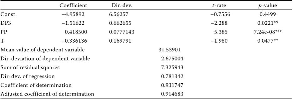
Table 4. Equation 3

Dependent variable: PAP

Const. –4.95892 6.56257 –0.7556 0.4499

DP3 –1.51622 0.662655 –2.288 0.0221**

PP 0.418500 0.0777143 5.385 7.24e-08***

T –0.336136 0.169791 –1.980 0.0477**

[image:6.595.63.532.593.751.2]

(7)

measured by the corrected coefficient of determina-tion is again relatively very high (R2 = 0.91).

The last explained variable at the producer level was the producer’s purchase price, that is the farmer price, where there was an anticipated influence of foreign prices, domestic prices of processing plants, and due to the course of the base values the equa-tion also included the time variable. The parameter estimates carried out are recorded in Table 4.

The quantification of the parameters first points out the negative impact of the dummy variable represent-ing the rate of import and export prices of beef, which means that the higher the import price is compared to the export price, the harder the imported products will probably be realized in the domestic market, which could, as a final result, be accompanied by an increase in the production capacity and a decrease in the purchase price. The intensity of the estimated parameter is very high, because a unit increase of

the used dummy variable would be followed by a decrease in the agricultural producer’s price by more than 1.5 units, ceteris paribus. On the other hand, an increase in the next explaining variable – the meat processing price – by a unit would induce an increase in the farmer price of 0.42 of a unit (ceteris paribus), which can be interpreted as an anticipated move-ment based on the strong dependence of producers on customers and on the existence of the motivation expectations. The negative value of the time vector is probably due to the relatively strong variations in the development of the farmer price, where there are visible time periods with stagnating prices which are subsequently repeatedly followed by a major drop.

[image:7.595.63.533.116.275.2]

From the statistical point of view, it can be stated that all parameters of explaining variables (except the automatically included constant) are statisti-cally significant at the selected level of significance (α = 0.05) and the proximity of dependence measured

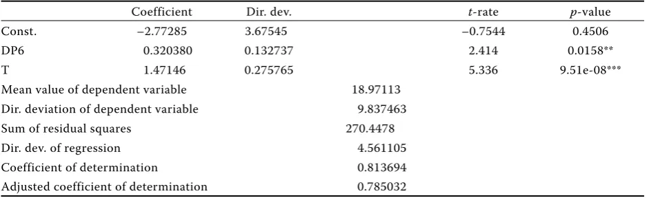
Table 6. Equation 5

Dependent variable: QEXD

Const. –2.77285 3.67545 –0.7544 0.4506

DP6 0.320380 0.132737 2.414 0.0158**

T 1.47146 0.275765 5.336 9.51e-08***

[image:7.595.63.534.608.752.2]

Table 5. Equation 4

Dependent variable: QIMD

Instrumental variable: const DP1 US T NMC DP3 DP6 TE CPP CPPL

Const. –85.7156 23.8409 –3.595 0.0003***

QDCD 0.290710 0.0712789 4.078 4.53e-05***

PP 0.495709 0.271163 1.828 0.0675*

T 1.97991 0.709886 2.789 0.0053***

(8)

by the corrected coefficient of determination is again relatively high (R2_{= 0.91).}

In the following stage, an estimate was made of the parameters of equations characterizing the foreign trade in beef. Table 5 contains the estimates of pa-rameters for the import equation and Table 6 contains the estimates of export parameters.

The performed estimate reached the expected values of parameters, which in the quantified model act in accordance with the factual logical verifica-tion. An increase in consumer demand by a unit would lead to an increase in import by 0.29 units, ceteris paribus, which probably corresponds to the fact that both domestic production and import of foreign products participate in meeting the domestic demand. An increase in the meat processing price of the chopped meat by a unit would probably, on the basis of the decreased price competitiveness of domestic production, allow for an increase in import by 0.49 units, ceteris paribus. The positive value of the time vector demonstrates the highly growing trend towards the import of beef to the Czech Republic.

From the statistical point of view, it can be stated that all parameters of the explaining variables are statistically significant at the selected level of signifi-cance (α= 0.05) excluding the parameter of the meat processing price, where the significance was proven at the level of α= 0.07, the proximity of dependence measured by the corrected coefficient of determina-tion is still very high (R2_=0.8).

Quantified in the export equation was the param-eter of another dummy variable which is formed by the rate of the export price and the domestic meat processing price. From the resulting value, it is ob-vious that an increase in the mentioned rate by one unit leads to an increase in export by 0.32 units, ceteris paribus, i.e. the higher value of the export price compared to the domestic meat processing

price should imply an increase in the export of beef, which can be regarded as a credible outcome of the economic principles of foreign trade based on the comparison of the domestic and foreign price levels similarly also in Kuhn (2004). The positive value of the time vector again demonstrates the sharply growing trend of export within the observed period, whilst it is possible on the basis of the parameter absolute value to identify an average year-to-year increase of 1.47 units, ceteris paribus.

The statistical assessment illustrates that both the explaining variables commented on are statisti-cally significant at the selected level of significance (α = 0.05). The inconsistent variable in the observed equation is the constant value. The proximity of de-pendence measured by the corrected coefficient of determination is still at a very high value (R2_{= 0.79).}

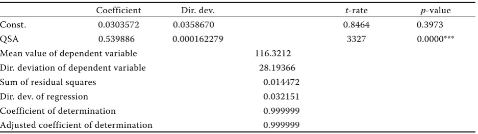
The meat processing level in the system is modelled first by the means of a simple dependence of domestic slaughter and domestic offer of slaughter animals, whose results are shown in Table 7.

The purpose of the quantified relation was to verify the theoretical value of the technological coefficient of the slaughter yield, which was achieved because the resulting value corresponds to the yield of ca 55%. The observed value will also be used in the further development of the conceived model beyond the scope of the presented paper.

The statistical verification for this equation is clear; its conclusiveness exceeds 99.9% probability, similarly to the proximity of dependencies, which is justifiably close to a deterministic relationship.

The Table 8 contains the estimated parameters of the equation explaining the offer of the chopped meat at the meat processing level.

[image:8.595.64.533.619.751.2]

The achieved values of the parameters are conflicting from the point of the economic verification, because the quantity of imported beef increases the domestic

Table 7. Equation 6

Dependent variable: DS

Const. 0.0303572 0.0358670 0.8464 0.3973

QSA 0.539886 0.000162279 3327 0.0000***

(9)

meat processing offer (one unit increase of import implies an increase in the offer by 1.23 units, ceteris paribus) and on the contrary, one unit increase of the meat processing price would induce a drop in the meat processing plant offer of the chopped meat by 0.4 units, ceteris paribus. The negative parameter of the price can, however, be neglected because it is not conclusive according to the statistical verification – see the p-value of the applied t-test. The positive influ-ence of the statistically significant (α= 0.05) import of beef, which is not a part of the meat-processing offer in the model structure, can be interpreted only partly, in cases of the import of live animals or whole carcasses or halves which are subsequently processed in the territory of the Czech Republic and contribute to the increase in the domestic processed meat offer. A similar conclusion was arrived upon by e.g. Istudor et al. (2007) during simulations of the influences affect-ing pig slaughter. The stated facts must be subjected

to a further observation of the commodity structure of foreign trade, which is not the subject or purpose of the presented paper. From the statistical point of view, the fact that there is a very low proximity of dependence (R2 _{= 0.2) in the given function is an} indicator that the conceived relation provides only a limited compliance with the base data and it should be subjected to a more complex analysis in further examination as well as to modifications, mainly in the sense of the inclusion of delayed variables.

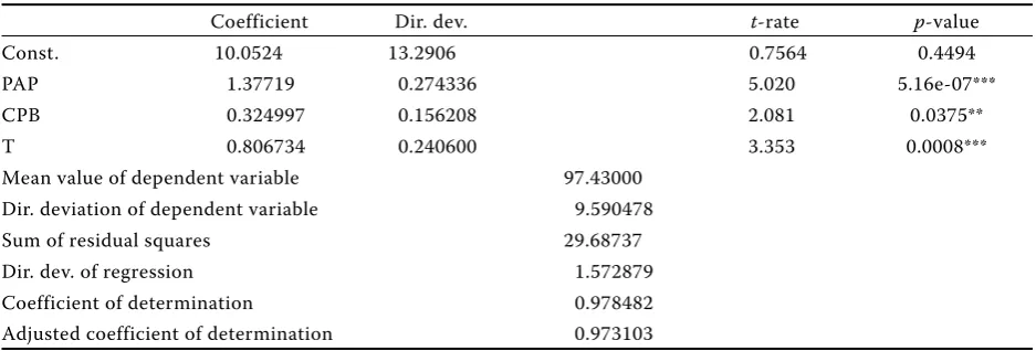
Conceived at the level of the meat processing in-dustry was an equation representing the influence of determinants of the industrial producer price, that is, the processed meat prices (Table 9).

[image:9.595.66.533.118.262.2]

The interpretation of the quantified parameters corresponds to the economic expectations. The agricultural producer’s price has a very strong in-fluence on the explained variable, because a one unit increase in the farmer’s price increases the Table 8. Equation 7

Dependent variable: QSP

Const. 177.757 40.6238 4.376 1.21e-05***

QIMD 1.22846 0.615851 1.995 0.0461**

PP –0.400540 0.471106 –0.8502 0.3952

Table 9. Equation 8

Dependent variable: PP

Const. 10.0524 13.2906 0.7564 0.4494

PAP 1.37719 0.274336 5.020 5.16e-07***

CPB 0.324997 0.156208 2.081 0.0375**

T 0.806734 0.240600 3.353 0.0008***

[image:9.595.63.532.591.750.2]

(10)

processed meat price by 1.3 units, ceteris paribus. Due to the processes of the price transmission the stated is expectable; although it points out that the increase in the price of the processed meat would be even higher than the original impulse. On the other hand, one unit increase in the consumer price would again induce an increase in the processed meat price, but only by 0.32 units (ceteris paribus), from which it is possible to assess the possible arrangement of the resulting consumer price and the proportion of the individual components, and indirectly also the negotiating power in the supplier-customer rela-tions. The last included variable was the time vec-tor, whose positive parameter demonstrates the long-term slightly growing value of the processed meat price. The statistical verification proves that all parameters of the explaining variables, except the

constant, are statistically significant at the selected level of significance (α= 0.05) and the proximity of dependence measured by the corrected coefficient of determination again increased to a relatively very high level (R2_{= 0.97).}

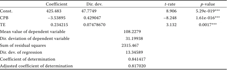
The penultimate stochastic equation of the specified commodity model explains the consumer demand for beef which depends on the consumer price for 1 kg of beef and on the amount of the average consumer expenses on meat (Table 10).

[image:10.595.64.531.117.261.2]

The results of the estimate provided are fully in compliance with the economic theory, because one unit increase in the consumer price would lead to a decrease in consumption by 3.54 units, ceteris paribus, which can be regarded as a very significant reaction, and from which it is possible to presume the high sensitivity of the Czech consumer to price

Table 10. Equation 9

Dependent variable: QDCD

Const. 425.483 47.7749 8.906 5.29e-019***

CPB –3.53895 0.429047 –8.248 1.61e-016***

TE 0.234215 0.07478670 3.132 0.0017***

Table 11. Equation 10

Dependent variable: CPB

Const. 28.2106 12.9207 2.183 0.0290**

PP 0.788390 0.0818459 9.633 5.82e-022***

CPP –0.109699 0.121098 –0.9059 0.3650

CPPL 0.317352 0.144093 2.202 0.0276**

DP3 2.64090 1.42901 1.848 0.0646*

[image:10.595.63.533.577.751.2]

(11)

levels of the observed goods. A similarly strong effect was arrived upon by, e.g., Zhao et al. (2000), whilst the results of the published research show that when similarly high price sensitivity is achieved with the basic needs goods, a state of saturation approaches and consumers are already unwilling to accept any increase in price or increase in offer. Consumer ex-penses on meat, which abstract a proportional part of the income which consumers allocate for their consumption of meat, have the expected positive effect – one unit increase in expenses creates an increase in consumption by 0.23 units, ceteris paribus. The direction and intensity of the effect is expected and it corresponds to the assumptions of the consumer behaviour theory.

From the statistical point of view, it can be stated that all parameters of the explaining variables are statistically significant at the selected level of sig-nificance (α = 0.01) and the proximity of dependence measured by the corrected coefficient of determina-tion is still very high (R2_{= 0.82).}

The last stochastic equation of the model is oriented on modelling of the consumer price to enable the analysis of mutual influences at the individual stages of the vertical. The consumer price is explained by the means of the processed meat price, the consumer price of pork and chicken and the dummy variable formed by the rate of the import and export price of beef (Table 11).

From the point of the observed results, it can be stated that one unit increase in the processed meat price would, ceteris paribus, increase the consumer price by 0.79 units, whilst the observed direction and intensity correspond to the assumptions. The consumer price of pork has a negative impact (one unit increase in the pork price would induce a de-crease in the price of beef at the consumer level of 0.1 units, ceteris paribus), and therefore it is possible to assume a rather complementary relation of both types of meat, probably due to their common

charac-teristics of red meat. However, that described above is more of an unconfirmed hypothesis, because the parameter of pork prices is not statistically conclu-sive. On the contrary, the parameter of the consumer price of poultry is conclusive; it has a positive ef-fect on the price of beef, and so the relation of beef and poultry can be regarded as competitive. One unit increase in the price of chicken would, ceteris paribus, induce an increase in the price of beef of 0.32 units. The conceived conclusion is backed by the different characteristics of both types of meat as well as by their completely different kilogram price in the spectrum of all meat types. Another possible reason is the ever-growing share of chicken in the meat semi-products at the cost of beef, most probably due to the price reasons. The last analyzed variable was the dummy formed by the rate of import and export prices of beef, whose increase by one unit would, under the condition of ceteris paribus, imply an increase in the consumer price of beef of 2.64 units. An increase in the import price compared to the export price would probably create a pressure on increasing the consumer price or it would create a certain space for it, respectively, and the mentioned effect would occur in a multiplied manner, appar-ently by the means of an increase in the price of the processed meat.

As has already been said earlier, the parameter of the pork consumer price was not detected as a statistically significant one, however, other quantified parameters are already significant at the level of significance of (α= 0.07). The proximity of dependence measured by the corrected coefficient of determination again reaches a high value of (R2_{= 0.93).}

For the summary recapitulation of the quantified relations, it is appropriate to note the resulting shape of the estimated simultaneous commodity model for beef in the Czech Republic in the form of equations (as the model was designed for the description of equilibrium, it necessarily includes a balance identity):

Q_SA,BM,t = 136.933 + 123.247NC_BM,t + 0.4126DP1 + 1.88225US – 10.6948T (62.04) (54.65) (0.197) (0.82) (2.87)

NC_BM,t = 1.71624 – 0.0023NMC_BM,t – 0.02PAP_BM,t + 0.0123US (0.19) (0.0003) (0.007) (0.003) PAP_BM,t = –4.95892 –1.51622DP3 + 0.4185PP_BM,t – 0.3361T (6.56) (0.66) (0.0777) (0.17)

Q_IMD,BM,t = –85.7156 + 0.29071Q_D,CD,BM,t + 0.4957PP_BM,t + 1.9799T (23.84) (0.071) (0.27) (0.71)

(12)

In the opening chapter of this performed analysis of estimated relations, there was a mention of the reference to the summary testing of econometric assumptions of the created model whose results are stated in the Tables 12, 13 and 14. In order to verify

the normal distribution of accidental components, a multi-criteria Doornik-Hansen test was chosen (Table 12) whose achieved p-value documents the confirmation of a zero hypothesis of normal distribu-tion of residuals in the conceived equadistribu-tions.

The verification of the non-presence of the autocor-relation of residuals was performed by the means of Table 12. Test for the multivariate normality of

residuals

Doornik-Hansen Chi-square(20) _{= 15.5703} With _{= 0.742901}p-value

Source: Own calculations

Table 13. Ljung-Box test (critical value = 0.05)

Equation 1:

Ljung-Box Q’: Chi-square(1) = 0.091569 [0.7622] Equation 2:

Ljung-Box Q’: Chi-square(1) = 0.61616 [0.4325] Source: Own calculations

Table 14. ARCH test (critical value = 0.05)

Equation 1:

ARCH test deg 1: P(Chi-Square(1) > 3.07256) = 0.0796242

Equation 2:

Equation 3:

Equation 4:

Equation 5:

Equation 6:

Equation 7:

ARCH test deg 1: P(Chi-Square(1) > 0.74045) = 0.389517 Equation 8:

Equation 9:

Equation 10:

Source: Own calculations DS_BM,t = 0.03 + 0.539886 Q_SA,BM,t

(0.036) (0.0002)

Q_SP,BM,t = 177.757 + 1.22846Q_IMD,BM,t – 0.40054PP_BM,t (40.62) (0.62) (0.47)

PP_BM,t = 10.0524 + 1.37719PAP_BM,t + 0.324997CP_BM,t + 0.8067T (13.29) (0.27) (0.156) (0.24) Q_DCD,BM,t = 425.483 + 3.53895CP_BM,t + 0.2342TE

(47.77) (0.43) (0.075)

CP_BM,t = 28.2106 + 0.78839PP_BM,t – 0.1097CP_PM,t + 0.3174CP_PLM,t + 2.6409DP3 (12.92) (0.082) (0.12) (0.14) (1.43)

(13)

a Ljung-Box test, whose simplified summary for all stochastic equations of the specified model is stated in Table 13.

On the basis of the comparison of the obtained p-values with the LB test critical value, it can be stated that the model is free of the autocorrelation of residuals.

Finally, also the heteroskedasticity was tested, by the means of a combined ARCH test. Since the previous LB test had already excluded the autocorrelation of residuals, it is possible to use an applied combined test for the verification which subsequently con-firms or rules out the hypothesis of homoscedasticity (Table 14).

From the results, it is obvious that not even for one tested equation is it possible to exclude the zero hypothesis of homoskedasticity, which confirms the compliance with the fundamental econometrical as-sumptions of the conceived model.

CONCLUSION

The examined market in beef has undergone sig-nificant changes in the observed period, which were determined by the economic development of our small open economy as well by several major shocks which significantly influenced the market structure as well as the mutual interactions within the vertical and reactions of the involved subjects to external impulses. When making a summary assessment of the general development of the basic levels of the observed vertical, it is necessary to state that the total offer at the level of the agricultural producer dropped by more than 47%, the numbers of cattle in the full-feed category dropped by more than 23%, whilst the unit subsidy for 1 kg of beef increased only by 3.15%. It is interesting from the point of view of the agricultural producer and the final consumer of beef products that the positive development in the maternal population of cows without market production, whose numbers in the surveyed period have increased more than five times. There has also been a growing trend in the farmer price, which, though, increased in the observed period only by 21%, which is an alarmingly low value given the in-crease in the prices of all inputs in the production. In comparison with the increase in the processed meat price (34%) and the consumer weighed price

(25%)2_{, the development of the price increase is not} proportional and there is an evidence of an enor-mous pressure mainly on the production stage of the vertical, due to which the development of the consumer price is probably still perceived by the end customers as adequate.

From the point of other basic characteristics, it is possible to state that in the observed period, there was a slight decrease in the offer of the chopped meat by ca 3% with a simultaneous decrease of the domestic slaughter by 53%, a sharp increase in import by 169% with a simultaneous increase of the import price by 377%, an increase in export by 160%, but with the export price only growing by 42%. Several partial conclusions can be conceived from the stated facts. The drop in production does not correspond to the drop in the numbers of cattle, which is ap-parently due to the increased import which makes up for the forced outages of Czech farmers, whose purchase prices are depressed to such a low level that for a number of subjects, the production is no longer profitable and there is a significant decrease in the numbers of cattle. It is also not good news for Czech consumers that balancing of the decreasing production base is achieved by the means of import with an extreme increase of the import price, which subsequently necessarily must determine the ad-joining links in the vertical. Last but not least, the increasing final prices need not be a consequence of the increasing prices at the production level but they may be caused by the behaviour of the foreign trade subjects who import products for high prices and on the other side, they probably export products with a low added value and with a very low increase in the export price.

At the consumer level, consumer expenses on meat in the observed period grew by 25%, but not due to an increase in the consumption of beef, which, on the contrary, dropped by 53%. The above-mentioned disproportion is due to the increase in the consumer price (of 25%, as already mentioned) and due to the fact that the observed data relates to all types of meat, that is, also chicken, which experienced a high increase in consumption.

During the analysis of the outputs of the conceived commodity model, some facts stated in the previous parts of the conclusions are confirmed and some partial results then provide support for other in-terpretations of relations in the examined vertical.

(14)

The model confirmed the decreasing trend of the farmer offer, which is, however, very sensitive espe-cially to increasing of the numbers of cattle, i.e. if the present decrease was stopped and the states of cattle possibly increased, the domestic production sector could very flexibly increase the production. A gradual increase in the unit subsidy would also sup-port the growth of the domestic production, although at the present development of the farmer price this serves more as a kind of brake on the otherwise sharp drop of the numbers of cattle and production. The decreasing numbers of cattle in the full-feed category unfortunately are not stopped even by the increasing numbers of the KBPTM, which together with the purchase price according to the calculated parameters have almost no influence on the total numbers and only prove the gloomy situation of Czech farmers. The agricultural producer price is surprisingly sensitive to the movements of the foreign trade prices, which, apparently due to the customers (meat processors), have a very strong position, giving further evidence of the positive influence of the processed meat price on the purchase price.

The significant increases in the import and export volumes are modified by the development of the rate between the domestic and foreign price as well as by the development of domestic consumption, as confirmed by the outputs of the estimated model. Both categories have a significantly positive param-eter of the time vector, whilst import would also be increased at an increase in the domestic demand as well as at an increase in the domestic processed meat price, which would make domestic products less competitive. Proven in the export equation were the standard economic principles, which increase export at increasing the rate of the export price compared with the domestic processed meat price. The total domestic offer of the meat processing sector is, ac-cording to the model outputs, strongly and positively influenced mainly by the realized import. The meat processing plant price is over-proportionally influ-enced by the farmer price and sub-proportionally pulled by the consumer price. The function of do-mestic consumption has the expected development, because an increase in the consumer price would induce a significant decrease in demand, and on the contrary, increasing income would slightly increase the demand. From the point of the consumer price, statistically significant influences of the processed meat price, the price of chicken and foreign trade prices were observed, whilst the industrial producer price increases the consumer price, similarly to the price of chicken, from which it is possible to assume the competitive relation between both types of meat.

Generally, it can be stated that the estimated model very well reflects the above analyzed principles of the examined vertical, declares the selected deter-minants of development of the offer and demand for beef as well as basic relations between the individual levels of the beef vertical, and therefore it can be regarded as a suitable tool for a subsequent analysis of the beef market and the subsequent simulation calculations.

REFERENCES

Cipra T. (2008): Finanční ekonometrie. (Financial econo-metrics .) 1st_{ed. Ekopress, Prague; ISBN} 978-80-86929-43-9.

Doornik J.A., Hansen H. (1994): An Omnibus Test for Univariate and Multivariate Normality. Working Paper, Nuffield College, Oxford.

Green W.H. (2008): Econometric Analysis. 6th_{ed. Pearson} Prentice Hall, New Persey; ISBN 978-0-13-513740-6. Gujarati D.N. (2003): Basic Econometrics. 4th_{ed. McGraw}

Hill, New York; ISBN 0-07-233542-4.

Hallam D. (1990): Econometric Modelling of Agricultural Commodity Markets. 1st_ed._{Routledge, London and New} York; ISBN 0-415-00405-5.

Istudor N., Manole V., Ion R.A., Pirjol T. (2007): Math-ematical model for optimizing the profit of the pork meat chain. Journal of Applied Quantitative Methods, 2: 507–516.

Kenedy P. (2008): A Guide to Econometrics. 6th_ed. Black-well Publishing, Oxford; ISBN 978-1-4051-8257-7. Kuhn A. (2004): Regional Agricultural Sector Model for

Ukraine. Working Paper No. 27. The Institute for Eco-nomic Research and Policy Consulting, Kiev.

Labys W.C., Pollak P.K. (1984): Commodity Models for Forecasting and Policy Analysis. 1st_{ed. Croom Helm} Ltd., London; ISBN 0-89397-193-6.

Lechanová, I. (2006): The transmission process of supply and demand shocks in Czech meat commodity chain. Agricultural Economics – Czech, 52: 427–435. Malý M., Kroupová Z. (2006): Efektivnost chovu

mas-ného skotu. (Efficiency of breeding cattle.) In: Sborník příspěvků z mezinárodní vědecké konference Agrarian perspectives XV – Foreign trade and globalisation pro-cesses. PEF, ČZU, Prague; ISBN 80-213-1531-8. Malý M. (2009): Price models in poultry meat vertical.

Scientia Ariculturae Bohemica, 2: 73–85

(15)

Nerlov M., Bessler D.A. (2001): Expectations, informa-tion and dynamics. In: Gardner B., Rausser G. (eds.): Handbook of Agricultural Economics, vol. I. Elsevier Science, Amsterdam.

Varian H.R. (1992): Microeconomic Analysis. 3rd_{ed. W.W.} Norton & Company Ltd., London; ISBN 978-0-393-95735-8.

Sarris A., Hallam D. (2006) (eds.): Agricultural Commod-ity Markets and Trade. FAO, Edward Elgar Publishing,

Cheltenham; ISBN 13:978-1-84542-444-2

Schaffer P. (2008): Commodity Modelling and Pricing. 1st_{ed. John Wiley & Sons,}_{New York;}_ISBN 978-0-470-31723-5.

SINE (1995–2010): Situační a výhledová zpráva hovězí maso. (Situation and Forecast Report – Beef.) Ministry of Agriculture CR, Prague; ISBN 978-80-7084-899-9.

SINE (1995–2009): Zpráva o stavu zemědělství. (General Information about Agriculture in the CR.) Ministry of Agricuture CR, Institute of Agricultural Economics and Information, Prague; ISBN (2009) 978-80-7084-940-8. SINE (1995–2009): Statistika rodinných účtů (Statistics of

Family Accounts). Czech Statistical Office, 1995–2009, Prague. Database source.

Zhao X., Mullen J.D., Griffith G.R., Griffiths W.E., Piggot R.R. (2000): An Equilibrium Displacement Model of the Australian Beef Industry. Economic Research Report No. 4, NSW Agriculture, Orange; ISBN 0-7347-1251-0.

Received: 30th_{December 2011} Accepted: 19th_{January 2013}

Contact address: