Mutation-Aware Fault Prediction
David Bowes
⇤, Tracy Hall
†, Mark Harman
‡, Yue Jia
‡, Federica Sarro
‡, and Fan Wu
‡⇤
University of Hertfordshire, Hatfield, UK
†Brunel University London, Uxbridge, UK
‡University College London, London, UK
ABSTRACT
We introduce mutation-aware fault prediction, which lever-ages additional guidance from metrics constructed in terms of mutants and the test cases that cover and detect them. We report the results of 12 sets of experiments, applying 4 di↵erent predictive modelling techniques to 3 large real-world systems (both open and closed source). The results show that our proposal can significantly (p 0.05) im-prove fault prediction performance. Moreover, mutation-based metrics lie in the top 5% most frequently relied upon fault predictors in 10 of the 12 sets of experiments, and pro-vide the majority of the top ten fault predictors in 9 of the 12 sets of experiments.
CCS Concepts
•Software and its engineering ! Software testing and debugging;
Keywords
Software Fault Prediction, Software Defect Prediction, Mu-tation Testing, Software Metrics, Empirical Study
1. INTRODUCTION
Software fault prediction1has been an active subject of re-search since the 1990s [12, 19, 22]. However, despite many proposals for di↵erent fault prediction techniques [4, 22, 66], no previous study has used mutation testing to improve the performance of predictive models.
In this paper we introduce mutation-aware fault predic-tion where several “mutapredic-tion metrics” – derived by using mutation testing – are used as features to build a fault pre-diction model. We term such a model a ‘mutation-aware’ predictive model.
The key insight motivating the consideration of mutation awareness is that fault prediction performance must surely 1Please note that both the termsfaultanddefecthave been used in the literature to refer to prediction models able to reveal faulty/defective software components.
depend on the ability of the test suite to find faults. This is because the performance of a prediction is measured as its ability to predict the faults that will subsequently be revealed (by testing). Since mutation testing is generally used to assess the e↵ectiveness of a test suite and previous work have demonstrated the coupling between real faults and mutation faults [3, 35], our motivation is to exploit this coupling: Mutation faults are coupled to real faults, so mu-tation faults should help predict real faults.
Consider the following scenario: The code has been tested by running a test suite, which may reveal some bugs. Unfor-tunately faults remain, we simply do not know where they reside; the dilemma faced by every tester. Our aim is to now predict where remaining faults are likely to reside. The majority of previous fault prediction studies has used static code metrics for this prediction task, yet there is dynamic information available resulting from the testing phase. The significant breakthrough of our study is that it is the first to use both static and dynamic test information. It is also the first to seed mutated faults which provides data allowing improved fault prediction.
In order to assess the e↵ectiveness of mutation-aware fault prediction we define 40 mutation metrics (either ‘static’ or ‘dynamic’) and collect them using the popular (and pub-licly available) tool PITest [14]. Then, we empirically com-pare the performance of mutation-aware prediction models built using these metrics with respect to those of prediction models built using 39 traditional (mutation-unaware) static source code metrics that have been widely used in previ-ous fault prediction work [46]. We also investigate whether the combined use of mutation metrics and source code met-rics improves the accuracy of the resulting prediction model. Moreover, we analyse the extent to which di↵erent predic-tion techniques benefit from mutapredic-tion awareness by using four di↵erent techniques (i.e., Logistic Regression, Random Forest, Na¨ıve Bayes and J48), implemented in WEKA [21], to build both ‘mutation-aware’ and ‘mutation-unaware’ pre-dictive models. Although we have our own tools for muta-tion testing and predictive modelling [26, 45, 50], we used publicly available third-party tools to avoid a source of po-tential experimenter bias, and to ensure that our results will have actionable findings for both mutation testing and pre-dictive modelling.
com-bined), are open-source systems widely used in fault predic-tion studies. We use both closed and open-source systems to increase the potential for generalisability, though of course, as with all studies of software systems, caution is required when extrapolating. Taken together, these systems consist of over 220K Lines of Code, with a total of 263 real world faultive classes, revealed by over 11K test cases.
To compare the performance of predictive models we use Matthews’ Correlation Coefficient (MCC), which has recently been demonstrated to be one of the most reliable measures of predictive model performance [70]. For compatibility with other studies on fault prediction, we also include Precision and Recall, which are widely used metrics to assess the prop-erties of predictive models.
The main contribution of this paper is the introduction of mutation-aware fault prediction, together with a study of the improvement mutation awareness conveys to fault pre-diction. The study involves 12 experimental evaluation sce-narios, consisting of 4 machine learners (predictive modelling techniques) and 3 real world systems for which ground truth fault data has been carefully collected.
Our primary finding is that mutation awareness can sig-nificantly improve predictive performance and with large ef-fect sizes. This is the first time any kind of mutation has been used to support fault prediction. Naturally, subsequent studies can further investigate/exploit this predictive im-provement, perhaps in combination with other sets of met-rics (e.g., process metmet-rics). In this first study we present the empirical evidence that mutation metrics e↵ect size on prediction outcomes can be large, thereby motivating and opening up this avenue of research.
In the following we briefly review the primary concepts underlying mutation testing and software fault prediction (Section 2). Then we present the research questions we aim to investigate (Section 3) and the design of the empirical study we carried out to answer them (Section 4). The re-sults of the study and threats to its validity are discussed in Sections 5 and 6, respectively. Section 7 summarises related work and Section 8 concludes.
2. BACKGROUND
2.1 Mutation Testing and Mutation Metrics
Mutation testing creates a variant of the program, called a mutant, into which a fault has been deliberately seeded [34]. Mutants are created by mutation operators, each of which seeds a particular class of faults, such as replacing one relational operator with another. A mutant is said to be ‘killed’ by a test case if the test case causes the original program and its mutant to behave di↵erently [34, 77].Originally, mutation testing was introduced in order to assess test e↵ectiveness [18, 38], but it has also been used as a technique to guide the generation of test cases [20, 26, 62], and to improve test oracles [20, 73]. One of the cornerstones of mutation testing is the hypothesis that at least some of the mutants will turn out to be coupled to real faults, such that test cases that are good at killing these mutants will also prove to be good at detecting real faults. There is empirical evidence to support this hypothesis [3, 35].
This paper introduces a new application: using mutation testing to guide fault prediction. We insert mutants into a program and collect metrics about them, not to assess or generate test cases or oracles, but in the hope that the
coupling between mutants and real faults will mean that at least some of these metrics will improve fault prediction.
We classify our mutation metrics as either ‘static’ or ‘dy-namic’. Static mutation metrics simply record the number of times a particular mutation operator can be applied, while dynamic mutation metrics record the number of times a par-ticular class of mutant is killed by the test suite (the mu-tation score for this class of mutants), and/or whether the mutant is executed (covered) by the test suite. Dynamic mu-tation metrics thus take account of the test suite as well as the potential faults that can be seeded, while static mutation metrics merely take account of the kinds of faults that can be seeded. We distinguish between the two because, should it turn out that static metrics improve fault prediction, then this benefit can be exploited even when no testing informa-tion is available. More details on the metrics collected are reported in Section 4.4.
2.2 Software Fault Prediction
A predictive model for software fault-proneness generally exploits past data about software modules to classify the software modules as either predicted faulty or predicted non-faulty. Predictive models infer a single aspect of the data (dependent variable) from some combination of other as-pects of the data (independent variables). In the software fault prediction context, the dependent variable is repre-sented by the faults contained in a software component while the independent variables may vary from project to project and can be related to di↵erent aspects of the software (e.g., source code metrics, process metrics).
The performance of the predictive model depends both on the modelling technique and the independent variables (i.e., metrics) used. Many predictive models have been in-vestigated in the literature. Among them, machine learners and regression algorithms such as Decision Trees, Logistic Regression and Na¨ıve Bayes are widely used [12, 36, 22]. Recently, also Search-Based approaches have been success-fully exploited (e.g., [1, 11, 25, 45, 68]). However, according to recent systematic literature reviews [22, 66], the choice of a modelling technique seems to have less impact on the clas-sification accuracy of a model than the choice of a metrics set. A selection of the most relevant variables (through fea-ture subset selection) from the set of variables contained in the original dataset can be performed to eliminate variables that are irrelevant or of no predictive information value, thus enhancing learning efficiency and increasing predictive accu-racy [22]. As the number of variables increases, finding an optimal feature subset might become intractable and di↵ er-ent strategies might be needed (e.g., greedy or search-based algorithms). Feature selection can be carried out by search-ing the space of variable subsets, evaluatsearch-ing each one [17]. This is usually achieved by combining a machine learning algorithm – used to evaluate the usefulness of the feature set – with a search method (i.e., wrappers). The feature selection can be done also by ranking methods (i.e., filters) that evaluate the features according to heuristics based on general characteristics of the data. These methods are based on statistics, information theory, or on some function of the classifier’s outputs.
faulty components incorrectly classified as non-faulty; False Positive (FP), non-faulty components incorrectly classified as faulty; True Negative (TN), non-faulty components cor-rectly classified as non-faulty. The confusion matrix values are used to calculate a set of evaluation measures. Typical ones are Precision (measuring the proportion of the compo-nents classified as faulty which are actually faulty), Recall (measuring the proportion of faulty components classified as faulty), and F-Measure (which is the harmonic mean of pre-cision and recall). However, it has been observed that these measures might be biased in the case of unbalanced data (i.e., minority and majority classes of very di↵erent sizes), which is often the case in fault prediction data. Thus, the use of balanced metrics, such as the Matthews Correlation Coefficient (MCC) has been recommended [70].
The MCC represents the correlation coefficient between the observed and predicted binary classifications and it is defined as follows:
M CC= p T P⇥T N F P⇥F N
(T P+F P)(T P+F N)(T N+F P)(T N+F N)
MCC values range between 1 and +1: +1 represents a perfect prediction, 0 no better than random prediction, and 1 indicates total disagreement between the prediction and the actual value. Contrary to other existing measures (e.g., Accuracy), MCC takes into account both true and false positives, and true and false negatives, so it is generally considered to be a balanced measure which can be used even if the data is unbalanced [70].
To validate predictive models across-validationprocess is typically used [4]. This process randomly splits the original dataset set into k-subsets (i.e., folds) of equal size (typi-cally,k=10). The model is trained by using the union ofk-1
subsets (i.e., a training set) and validated on the remaining one that represents the test set. The process is repeatedk
times, each time with a di↵erent testing set. In order to pre-vent overfitting an innerk-fold cross-validation can be also applied to the training set. To guarantee that the distribu-tion of the faulty and non-faulty instances into training and test sets is representative of the distribution of the original dataset, stratification can be also used in the cross-validation process. Stratification allows us to mitigate cases of unbal-anced data, such as using a fold with no faulty components, that might skew the result of the cross-validation process.
3. RESEARCH QUESTIONS
Our first research question investigates whether there is any e↵ect on the performance of predictive models when they use mutation metrics. Unless the answer to this ques-tion is ‘yes’, then there is no point in further investigating mutation-aware predictive modelling.
RQ1: Is the performance of predictive modelling techniques improved when they have mutation met-rics available?
In order to answer this research question we report on the di↵erence in predictive model performance when the predic-tive model has all of the 79 metrics available (the ‘with mu-tation metrics’ version), and when it only has available the 39 traditional metrics and no mutation metrics (the ‘with-out mutation metrics’ version). A 10-fold cross-validation is performed 50 times, each time with a di↵erent random shu✏e of the data, in order to account for the stochastic na-ture of the overall predictive modelling algorithm. We use a
two-tailed Wilcoxon non-parametric statistical test to check whether there are significant di↵erences in the means for the ‘with’ and ‘without’ mutation metrics performance. We use the Wilcoxon test because we have no evidence to suggest that the performance of the predictive models is normally distributed over 50 runs. We use a two-tailed test, because we make no assumptions about which version of the pre-dictive model will perform better in each case. We use the Matthews Correlation Coefficient (MCC), and Precision and Recall performance metrics to assess the predictive power of the fault prediction models.
If the answer to RQ1 is ‘yes’, then this motivates a more in-depth analysis of mutation metrics. However, an affi rma-tive answer to this question does not provide sufficient sci-entific evidence, on its own, to motivate the use of mutation-aware predictive modelling. It could be, for example, that mutation metrics only very occasionally improve the perfor-mance of a predictive modelling technique, or that they im-prove the performance more often, but only by a very slight amount. If the e↵ect is too infrequent, or the size of e↵ect too small, then there will still be no point in further study of mutation-aware predictive modelling. This motivates a second research question below:
RQ2: What is the e↵ect size of improvements in predictive model performance due to mutation met-rics?
We split this overall research question into three sub ques-tions, which ask about the frequency and size of the e↵ects of mutation testing on predictive modelling performance.
RQ2.1: What is the frequency with which each pre-dictive modelling technique uses mutation metrics?
Using the same validation approach as for RQ1, we ex-plore the results of the nested feature subset selection, for the four machine learners considered in this study. There-fore, for each subject and each learner, we obtain 500 di↵ er-ent probabilistic model instances (50 repetitions of 10-fold cross-validation), each of which has its own set of metrics, identified by feature subset selection. For each of the 79 metrics, we record which of the metrics occurs in these 500 probabilistic model instances. This frequency gives one in-dication of the importance of each metric, in terms of how often it is selected by feature subset selection, for each algo-rithm on each subject system. If some of the mutation met-rics occur very frequently, then this strengthens the scientific evidence for the positive influence of mutation awareness on fault prediction.
RQ2.2: When a predictive modelling technique uses a mutation metric, what is the average predictive performance improvement due to this metric?
A particular metric may be frequently selected, yet with little e↵ect on each occasion. Therefore, evidence for the frequent use of mutation metrics is encouraging, but insuf-ficient on its own, to support strong scientific claims for mutation-aware predictive modelling. We therefore further investigate, by complementing the results of RQ2.1 with a study of the e↵ect size for each of the mutation metrics: how much does it a↵ect the predictive model performance on each occasion when it is used?
each metric when this is selected during the feature subset selection phase of each of the algorithm considered.
RQ2.3: For each mutation metric used on any occa-sion by a predictive modelling technique, what is the overall contribution of the metric to performance improvement?
Some metrics may have a big e↵ect when they are used, but may, nevertheless, still be infrequent over all predictive model instances (i.e., such metrics are very useful, but only on a few occasions). If all the mutation metrics fall into this category, then that would be interesting, but would not constitute strong scientific evidence for mutation-aware fault protection. In order to capture the overall influence of each metric on the predictive models, we report on the product of the frequency and the e↵ect size. This measures the average overall e↵ect of a particular metric over all instances of a predictive modelling algorithm and subject system.
If we find that mutation metrics are selected frequently by feature subset selection, and that they can have a big e↵ect when they are deployed into a predictive model, and that overall, their e↵ect size is large, then we will have strong overall scientific evidence for the value and importance of mutation-aware fault prediction. We can then move on to study the individual mutation metrics (and classes of met-rics) in more detail, which we do in RQ3 below.
RQ3: What is the relative performance of static and dynamic mutation metrics? In order to answer this question, we twice repeat the experimental procedure used for RQ1; once for static mutation metrics, and once for the dynamic mutation metrics. This allows us to inves-tigate the individual specific advantage conveyed to predic-tive modelling using each of these sets of mutation metrics to complement the existing source code metrics.
Static mutation metrics can be computed in the absence of any test data, while dynamic mutation metrics also require a test suite. It is therefore interesting to see whether mutation metrics can benefit predictive modelling performance, even in the absence of a test suite; are static mutation metrics useful in their own right? We might expect that dynamic mutation metrics would convey greater advantage to a pre-dictive modelling algorithm than static mutation metrics, because they also imbue the model with information about the test suite. If this is the case, then it suggests that other ‘test suite aware metrics’ might be investigated for their pos-itive e↵ects on fault prediction. On the other hand, it will be surprising and interesting if we find that such test suite information is not beneficial to fault prediction.
4. EXPERIMENTAL SETUP
In order to support replication2, this section provides de-tails of the subject systems and their fault data, the source code and mutation metrics we used and the predictive mod-elling techniques with which we experimented.
4.1 Subject Systems
Table 1 provides details of the three subject systems used in this study. We can observe that there is variation in the size of the systems as well as the proportion of faulty classes 2The data used in this study (except for the closed source TelCom system which is covered by a Non-Disclose Agreement) is available at http://www0.cs.ucl.ac.uk/sta↵/F.Sarro/projects/
faultPrediction/index.html.
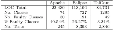
Apache Eclipse TelCom LOC Total 22,430 113,106 84,731
No. Classes 74 727 1295
No. Faulty Classes 30 191 42
% Faulty Classes 40.54% 26.27% 3.24%
[image:4.612.339.524.66.115.2]No. Tests 245 8,393 2,846
Table 1: Contextual Information for the Subject Systems.
in each. The TelCom system has a very low proportion of faulty classes (3.24%) making it a difficult subject for which to build good fault prediction models. Apache has the highest proportion of faulty classes at 40.54%. Table 1 also shows that the number of tests used varies across the three systems. Apache has the lowest number of tests at 245 which may explain the relatively high faultiness in Apache.
4.2 Fault Data
We collected fault data from each of the three subject systems using the ´Sliwerski, Zimmerman and Zeller (SZZ) algorithm [71]. The SZZ algorithm matches the fault fix de-scribed in the bug tracking system with corresponding com-mits in the version control system that fixed that fault. This means that we were able to identify the fault insertion and fix points for every class in each of the subject systems and to label each class as either faulty or not-faulty for a given point in time. The data we collected has already been used in our previous work [23], where more details are provided.
4.3 Source Code Metrics
We collected 39 source code metrics (see Table 2) from each of the three subject systems. These metrics are wide-ranging and are frequently used in fault prediction studies [22]. We collected these metrics using the default settings of JHawk 1.8 [74], a tool previously identified as robust for collecting source code metrics from Java systems [46].
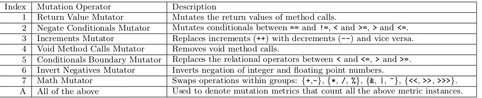
4.4 Mutation Metrics
Index Mutation Operator Description
1 Return Value Mutator Mutates the return values of method calls.
2 Negate Conditionals Mutator Mutates conditionals between==and!=,<and>=,>and<=. 3 Increments Mutator Replaces increments (++) with decrements (--) and vice versa. 4 Void Method Calls Mutator Removes void method calls.
5 Conditionals Boundary Mutator Replaces the relational operators between<and<=,>and>=. 6 Invert Negatives Mutator Inverts negation of integer and floating point numbers.
[image:5.612.65.548.65.164.2]7 Math Mutator Swaps operations within groups: {+,-},{*,/,%},{&,|,^},{<<,>>,>>>}. A All of the above Used to denote mutation metrics that count all the above metric instances.
Table 4: Mutation Operators
Coding Meaning Origin
AVCC Average Cyclomatic Complexity [47] CBO Coupling Between Object Classes [13] CCML Cumulative Number of Comment Lines [74] CCOM Cumulative Number of Comments [74]
COH Cohesion [13]
DIT Depth of Inheritance Tree [13]
EXT External Method Calls [74]
F-IN Fan In [29]
FOUT Fan Out [29]
HBUG Halstead Cumulative Bugs [24]
HEFF Halstead E↵ort [24]
HIER Hierarchy Method Calls [15]
HLTH Halstead Cumulative Length [24] HVOL Halstead Cumulative Volume [24]
INST Instance Variables [74]
INTR Number of Interfaces [74]
LCOM Lack of Cohesion of Methods [13] LCOM2 Lack of Cohesion of Methods version 2 [13]
LMC Local Method Calls [74]
MAXCC Max Complexity [74]
MI Maintainability Index [61]
MINC Maintainability Index (No Comments) [61]
MOD Number of Modifiers [47]
MPC Message Passing Coupling [42]
NCO Number of Commands [74]
NLOC Lines Of Code
NOM Number of Methods [74]
NOS Number of Statements [74]
NQU Number of Queries [74]
NSUB Number of Subclasses [13]
NSUP Number of Superclasses [74]
PACK Number of Imported Packages [74]
R-R Reuse Ratio [69]
RFC Response For class [13]
S-R Specialization ratio [69]
SIX Specialization index [44]
Superclass SuperClass Name [74]
TCC Total Complexity [47]
UWCS UnWeighted Class Size [74]
Table 2: JHawk[74] Source Code Metrics Used (www.virtualmachinery.com/jhawkmetricslist.htm).
4.5 Machine Learning Techniques
In this study we used four di↵erent classifiers (i.e., Na¨ıve Bayes, Logistic Regression, J48, Random Forest) which cover a range of di↵erent techniques. Na¨ıve Bayes (NB) [76] is a statistical technique which uses the combined probabilities of the di↵erent attributes to predict faultiness. Logistic Re-gression (LR) [16] is a reRe-gression technique which identifies the best set of weights for each attribute to predict the bi-nary class. J48 is a Java implementation of the C4.5 [65] decision tree algorithm which uses entropy information to determine which attribute to use as decision nodes. Random Forest (RF) [9] is an ensemble technique which aggregates the predictions made by a collection of decision trees (each with a subset of the original set of attributes).
For each of these techniques we used the WEKA Wrapper Subset Selection Filter [40, 21] which performs a best first
Metric Description Type
MuNOMS Number of generated mutants Static MuNOC Number of mutants covered by tests Dynamic
MuNNC Number of mutants not covered by tests Dynamic
MuMS Mutation score of generated mutants Dynamic
MuMSC Mutation score of covered mutants Dynamic
Table 3: Mutation metrics considered in our study.
Key to colours/shading: Metrics inblue(dark grey for those reading a b/w copy) are static mutation metrics, while those inboldfaceare dynamic mutation metrics.
search algorithm to identify the subset of attributes that generalise best on the training set.
In order to validate the approaches we performed a 10-fold cross validation with an inner 5-10-fold cross-validation on the training set, and evaluated the results using MCC (see Section 2).
5. RESULTS
Our base results using only static code metrics are com-parable if not better than results from other studies. Previ-ous fault prediction work on Eclipse data, using static code metrics reported an average MCC of 0.412 with a standard deviation of 0.150 [22]. Our Eclipse results with static code metrics have an average MCC of 0.447 indicating that any improvement using mutation metrics improves even further than the majority of previous studies.
RQ1: Do Mutation Metrics Improve Performance?
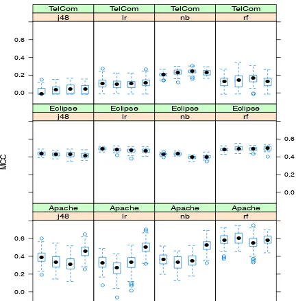
Figure 1 contains three rows, each of which corresponds to one of the three subjects systems. Within each row, each of the four sets of box plots corresponds to one of the four di↵erent learning algorithms. Within each set there are box plots, labelled C, S, D, and A, which correspond to the MCC values obtained by the predictive models built using source code metrics alone, source code metrics augmented by static mutation metrics, source code metrics augmented by dy-namic mutation metrics, all metrics (source code metrics augmented by static and dynamic mutation metrics)
MCC
0.0 0.2 0.4 0.6
C S D A
● ● ● ● ● ● ● ● j48 Apache
C S D A
● ● ● ● ● ● ● ● ● ● ● ● ● lr Apache
C S D A
● ● ●
●
●
nb Apache
C S D A
[image:6.612.68.284.76.295.2]● ● ● ● ● ● ● ●● ● ● ● ● rf Apache ● ● ● ● j48 Eclipse ● ● ● ● ● ● lr Eclipse ●● ● ● ● ● ● nb Eclipse 0.0 0.2 0.4 0.6 ● ● ● ● ● ● rf Eclipse 0.0 0.2 0.4 0.6 ● ● ● ● ● j48 TelCom ● ● ● ● ● ● lr TelCom ● ● ● ● ● ● ● ● ● ● nb TelCom ● ● ● ● ● ● rf TelCom
Figure 1: RQ1 and RQ3: MCC values for di↵erent predic-tive modelling algorithms on each of the three subjects. Key:
nb=Na¨ıve Bayes,lr=Logistic Regression,rf=Random For-est,j48=J48; C: source code metrics alone, S: source code metrics augmented by static mutation metrics, D: source code metrics augmented by dynamic mutation metrics, A: all metrics (source code metrics augmented by static and dynamic mutation metrics).
of any of the four algorithms, whether with or without mu-tation awareness. Furthermore, for Eclipse, all approaches to predictive modelling appear to show very little variance. To further analyse these results, we performed an infer-ential statistical analysis of the di↵erences between the me-dian MCC values observed for each technique, the results of which are presented in Table 5a. These results confirm that fault prediction for the Apache system significantly benefits from mutation awareness. The industrial TelCom system also benefits from it, however the improvement is less pro-nounced. For the Eclipse system, there is a small reduc-tion in performance, using mutareduc-tion aware metrics. After performing the Benjamini-Hochberg correction for multiple statistical testing [5], onlyp-values <0.001 remain signifi-cant.
Tables 5b and 5c provide a comparison of the di↵erences (and their statistical significance) for the Precision and Re-call values obtained using source code metrics alone, and using source code metrics augmented by mutation metrics (both static and dynamic). The results are consistent with those for the MCC performance metric. The Precision and Recall values give a more detailed explanation of the dra-matic improvement achieved in MCC for the Apache system. Figure 2 shows the box plots of Precision and Recall values for this system. We can observe that mutation awareness improves the Recall of the predictive models, while retain-ing their Precision. As a result, more faulty classes are cor-rectly identified using mutation metrics, without introduc-ing any extra false positives (false alarms). The improve-ment in Recall for di↵erent systems results in being able
to correctly predict additional faults: Apache with Na¨ıve Bayes +7 (50%), Eclipse with Random Forest +2 (2%) and TelCom with Na¨ıve Bayes +1 (9%).
(a) MCC
Apache Eclipse TelCom
Na¨ıve Bayes <0.001 (0.182)
<0.001
(-0.030)
0.018
(0.022) Logistic Regression <0.001
(0.164)
<0.001
(-0.020)
0.338 (0.005)
Random Forest 0.858 (-0.008)
0.005
(0.013)
0.920 (0.000)
J48 <0.001
(0.070) <0.001 (-0.019) 0.007 (0.057) (b) Precision
Apache Eclipse TelCom
Na¨ıve Bayes 0.049 (0.032)
0.020
(-0.009)
0.195 (0.009) Logistic Regression <0.001
(0.085)
<0.001
(-0.019)
0.871 (0.000)
Random Forest <0.001 (-0.028) 0.009 (0.012) 0.768 (-0.013) J48 0.008 (0.026) <0.001 (-0.025) <0.001 (0.143) (c) Recall
Apache Eclipse TelCom
Na¨ıve Bayes <0.001 (0.267)
<0.001
(-0.039)
<0.001
(0.024)
Logistic Regression <0.001 (0.167)
<0.001
(-0.016)
0.033
(0.000) Random Forest <0.001
(0.067)
0.023
(0.010)
0.317 (0.000)
J48 <0.001
(0.100)
0.681 (-0.008)
<0.001
[image:6.612.312.536.103.442.2](0.024)
Table 5: Two-tailed Wilcoxon test results arep-values that show the probability that we would obtain the di↵erence in medians we observe, if the mutation metrics were to have no significant e↵ect on predictive performance measured using MCC (a), Precision (b), and Recall (c). The number in brackets is the di↵erence between the median values; where it is positive, it indicates that mutation metrics can improve predictive performance.
In conclusion, we find evidence that mutation awareness can improve the performance of predictive modelling, and that improvement is not restricted to only one technique, but can improve multiple techniques. There is also evidence that, where it does provide an improvement, the e↵ect is highly significant. We therefore find evidence that mutation awareness is beneficial to predictive modelling.
RQ2: What is the e↵ect size of improvements in predictive model performance due to mutation met-rics? Having found evidence that mutation awareness can benefit predictive modelling, we now turn to a more detailed analysis of the frequency and (local and global) e↵ect sizes of this benefit.
RQ2.1: What is the frequency with which each pre-dictive modelling technique uses mutation metrics?
0.3 0.4 0.5 0.6 0.7 0.8 0.9
C S D A ● ● ● ● ● ●
j48 Precision
C S D A ● ● ● ● ● ● ● lr Precision
C S D A ● ● ● ●
● ●
nb Precision
[image:7.612.322.540.62.432.2]C S D A ● ● ● ● ● ● rf Precision ● ● ● ● ● ● ● ●● ● ● ● ● ● ● j48 Recall ● ● ● ● ● ● ● ● ● ● ● ● lr Recall ● ● ● ● ● ● ● ● nb Recall 0.3 0.4 0.5 0.6 0.7 0.8 0.9 ● ● ● ● ● ● ● ● rf Recall
Figure 2: RQ1.Precision and Recall for Apache.
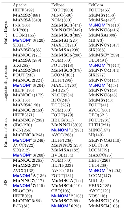
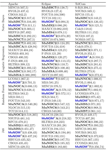
software systems). The number in brackets after each muta-tion name indicates the number of times (out of 500 folds in the cross fold validation) that the metric was used (for ex-ample, a number above 250 indicates that the corresponding metric is more likely to be used than not). We can observe that mutation metrics are very prevalent in every one of the 12 experiments, indicating that they are frequently useful in all of the predictive modelling scenarios considered. Table 7 gives a count of the number of mutation metrics that occur in the top 10 for each of the 12 experiments. As can be seen, the mutation metrics make up 50% or more of the top ten fault-predicting metrics for most cases and occur in the top 5% (4/79) fault predictors in 10 of the 12 sets of experi-ments. Also, in every case (except 3: Random Forests (RF) applied to TelCom and J48 applied to Eclipse and TelCom) there is at least one mutation metric that is more likely to be used than not.
The results are also revealing for the traditional source code metrics: For example, our results provide evidence to suggest that di↵erent systems and di↵erent algorithms require di↵erent source code metrics for best performance. Clearly, the ‘Fan Out’ metric (FOUT) is highly applicable in many cases, being the most popular of all 79 metrics in 3 of the 12 experiments. Nevertheless, even this apparently useful metric, plays no role in the top 10 results for the J48 algorithm for any of the three systems studied. This find-ing, for traditional metrics, underscores the difficulty of fault prediction in general, and the impossibility of finding uni-versally applicable techniques that always improve all fault predictions [72]. This observation tends to suggest that the scientific evidence for mutation awareness is all the more compelling, since it is so consistently beneficial to so many instances of the predictive modelling algorithms.
RQ2.2: When a predictive modelling technique uses a mutation metric, what is the average predictive performance improvement due to this metric? From RQ 2.1, we know that mutation metrics frequently provide benefit to all the predictive modelling algorithms and for all the programs studied. However, Table 7 simply consid-ered the frequency with which a metric was used; this says nothing about the size of the e↵ect, to which we now turn. Table 8 shows the e↵ect size of the top ten (out of 79)
met-Apache Eclipse TelCom
Na ¨ıv e Ba y es
HEFF(492) FOUT(500) FOUT(465)
MuMS2(488) MINC(500) MuMS7(458)
MuMSA(340) NOM(500) MuMS4(427) R-R(306) MuMSC4(471) MuNOMS7(418)
MI(266) MuNOC2(342) MuNNC3(416)
LCOM(155) MuMSC3(309) MuMSA(398)
MuNOMS3(120) MuMS1(226) MI(373)
SIX(117) MAXCC(210) MuNNC7(317)
MuMSC3(85) MuMSA(209) SIX(268)
MuNOC7(71) MuMSC5(206) MuMSC7(259)
L o g is ti c R eg re ss io n
MuMSA(289) NOM(500) CBO(494)
SIX(285) FOUT(418) MuNOMS7(443)
MuMS2(284) MuMSC3(378) MuNNC4(314)
FOUT(233) LCOM(303) SIX(277)
MuNOC2(224) HEFF(296) MuNNC5(147)
MuNOMS3(204) MAXCC(263) MuNOMS4(58)
HEFF(195) R-R(257) MuNNC7(49)
MuNOC1(172) NLOC(254) MuNNC3(45)
R-R(136) RFC(248) MuMS7(43)
MuMS4(128) TCC(237) FOUT(41)
R a ndo m F o re st
MuNOC2(463) NOM(500) AVCC(500)
HEFF(371) FOUT(479) CBO(321)
MuNNC7(285) HBUG(311) FOUT(234)
CBO(270) MuNNC1(309) HLTH(221)
F-IN(266) MuNOMS1(295) MINC(157)
MuNNC3(263) AVCC(288) MI(149)
MuNOMS4(246) HEFF(238) MuNNCA(110)
AVCC(222) MuNNC2(238) NLOC(80)
SIX(212) MuMSA(182) LCOM(79)
MuNOMS3(200) HVOL(134) MAXCC(75)
J48
MuNOC2(265) NOM(500) HEFF(226)
MuMS2(227) HLTH(223) CBO(209)
AVCC(138) AVCC(151) MuNOMSA(202)
MuNOMSA(136) FOUT(131) LCOM(147)
MuNNC7(117) MuMSCA(122) MI(142)
MuNOMS7(115) MuMSC4(119) HBUG(135)
NLOC(92) CBO(106) AVCC(129)
HEFF(89) MuNOMS2(105) NOS(116)
MuNNC3(86) MuMSC7(99) MuMSC1(105)
F-IN(81) MuNOMS6(96) MuMSC4(105)
Table 6: RQ2.1. Top 10 most frequently used metrics for di↵erent datasets and classifiers.
rics in terms of their ‘local’ contribution to the performance of the algorithm. This e↵ect size is ‘local’ in the sense that we measure the e↵ect on the MCC performance assessment, only when the particular metric concerned is used.
Since MCC values lie between minus one and one, any improvement above 0.1 can be considered to be large and anything above 0.2 to be very large. For example, an im-provement above 0.2 would be larger than the imim-provement that could be gained byanyof the four algorithms onanyof three systems studied, using the traditional source code met-rics. As Table 8 reveals, when a mutation metric is used, its e↵ect on the performance of the predictive model that uses it can be extremely large. In all but 1 of the 12 experiments, the e↵ect size of at least one mutation metric is above 0.1.
Technique Apache Eclipse TelCom
Na¨ıve Bayes 5 6 7
Logistic Regression 6 1 7
Random Forest 5 4 1
[image:7.612.75.284.80.239.2]J48 6 5 3
[image:7.612.330.533.621.675.2]Apache Eclipse TelCom
Na
¨ıv
e
Ba
y
es
MINC(0.507,5) MuMSC7(0.138,7) S-R(0.394,1) HVOL(0.437,4) HVOL(0.127,4) NSUB(0.349,1) CBO(0.342,2) FOUT(0.104,500) RFC(0.155,4)
MuNOC2(0.317,4) TCC(0.102,11) MuMSC1(0.143,2)
MuMSC7(0.316,49) MuNOMS5(0.094,3) MuNOC4(0.126,45)
MuNOMS7(0.311,1) MuMS2(0.086,28) MuNOMS5(0.121,5)
MuNOC1(0.303,1) MAXCC(0.082,210) Coh(0.118,6)
HEFF(0.297,492) MuMS4(0.078,11) HLTH(0.111,152)
MuMSC1(0.292,21) MuNOMS2(0.074,20) NCO(0.107,2)
MuNNC7(0.287,5) MINC(0.074,500) NOM(0.107,5)
L
o
g
is
ti
c
R
eg
re
ss
io
n
MuMSC7(0.482,16) MuMSC2(0.124,29) MuNNC2(0.384,2)
MuMSCA(0.428,94) FOUT(0.124,418) Coh(0.379,1)
MAXCC(0.404,24) MuMS4(0.123,21) MuMSC2(0.371,1) NOM(0.403,16) F-IN(0.121,29) HVOL(0.352,1) CBO(0.400,33) MuMS2(0.120,27) MuNOMSA(0.316,2)
F-IN(0.400,13) MuNOMS6(0.113,15) MuNNC1(0.287,7)
HLTH(0.399,12) MuNNC6(0.110,7) MuMSC1(0.281,6)
MuMSC2(0.393,12) MuNNC2(0.100,46) MuNOC5(0.275,4)
MuMSC1(0.382,17) MuMSA(0.099,40) HLTH(0.273,9)
MuMSA(0.380,289) AVCC(0.097,83) MuNOMS5(0.272,8)
R
a
ndo
m
F
o
re
st
LCOM(1.067,2) MuNOMS7(0.687,1) MuNNC6(1.006,8)
MuNOMS2(0.701,3) MI(0.581,25) HVOL(1.004,4)
MuNOCA(0.686,13) MINC(0.576,5) MuNOMS2(1.002,8)
MuNNC1(0.638,4) MuNOMSA(0.576,12) MuMSC7(1.002,9)
HLTH(0.583,2) MuNOMS2(0.572,11) LCOM2(0.978,11)
MI(0.583,1) SIX(0.564,7) MuMS2(0.975,42) FOUT(0.543,10) F-IN(0.549,13) MuNOMS5(0.971,17)
MuNNCA(0.540,26) MuNOC3(0.547,12) MuMS5(0.971,33)
NLOC(0.515,13) MuNNC6(0.543,21) MuNOC6(0.968,3) TCC(0.514,11) CBO(0.543,80) MuMS7(0.961,14)
J48
MuNOC2(0.518,265) NLOC(0.238,54) HVOL(0.449,17)
NSUP(0.481,14) MuNOMSA(0.218,32) TCC(0.407,28)
RFC(0.479,21) HLTH(0.218,223) MuNOC3(0.396,22)
MuMS2(0.462,227) MAXCC(0.201,28) MuNNC7(0.393,22)
MuMS5(0.451,27) AVCC(0.194,151) MINC(0.383,30)
MuNOMS1(0.438,43) MuNOCA(0.194,48) NSUB(0.383,32)
MuNOMS3(0.437,24) FOUT(0.193,131) MuNNC1(0.372,63)
HBUG(0.435,32) MuMSC3(0.187,75) HBUG(0.367,135) CBO(0.435,45) MuNOC5(0.185,32) CCOM(0.363,53) MINC(0.429,55) MuMS3(0.183,60) MuNOMS7(0.356,74)
Table 8: RQ2.2. Contribution of metric towards MCC(training) when using Na¨ıve Bayes, Logistic Regression and J48.
These results suggest that where a mutation metric is used, its e↵ect on the performance of a predictive model is large. However, these results cover only the local e↵ect size, so we now study the global e↵ect sizes in RQ2.3.
RQ2.3: For each mutation metric used on any oc-casion by a predictive modelling technique, what is the overall contribution of the metric to perfor-mance improvement? Table 9 shows the e↵ect size of the top ten (out of 79) metrics in terms of their ‘global’ con-tribution to the performance of the algorithm. This e↵ect size is ‘global’ in the sense that we measure the e↵ect on the MCC performance assessment, across every use of the metric, counting its e↵ect as 0.0 for all folds that fail to use it. As can be seen from the table, mutation metrics have a high global e↵ect size in many cases. In 9 out of the 12 experiments, more than half of the top 10 global e↵ect size metrics are mutation metrics. For the Apache system, there is a mutation metric that has a large e↵ect size ( 0.2) for all four algorithms studied. For the other two systems, the e↵ect sizes are lower for the mutation metrics, but they are also lower for all metrics overall, indicating that, for these systems, there is seldom a single metric that can have a big impact on its own.
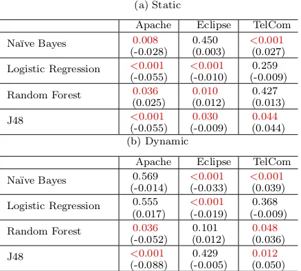
RQ3: What is the relative performance of static and dynamic mutation metrics?
Consider again, Figures 1 and 2, which we used to answer RQ1. Each figure also reports results for the separate ef-fect on predictive model performance of static and dynamic
Apache Eclipse TelCom
Na
¨ıv
e
Ba
y
es
HEFF(0.292,492) FOUT(0.104,500) FOUT(0.094,465)
MuMS2(0.252,488) MINC(0.074,500) MuNNC3(0.056,416)
MuMSA(0.152,340) MuMSC4(0.046,471) MuMS7(0.055,458)
MI(0.073,266) MAXCC(0.034,210) MuMSA(0.055,398) R-R(0.063,306) MuNOC2(0.029,342) MuMS4(0.054,427) LCOM(0.042,155) NOM(0.025,500) SIX(0.051,268) MuNOMS3(0.036,120) MuMS1(0.023,226) MuNOMS7(0.049,418)
MuMSCA(0.033,66) MuMSC3(0.021,309) MI(0.047,373)
MuMSC7(0.031,49) MuMS6(0.018,254) MuNNC4(0.042,225)
MuMSC3(0.021,85) MuMSC5(0.018,206) CBO(0.036,238)
L
o
g
is
ti
c
R
eg
re
ss
io
n
MuMSA(0.220,289) FOUT(0.103,418) MuNNC4(0.085,314)
MuMS2(0.212,284) NOM(0.069,500) CBO(0.078,494)
SIX(0.189,285) MuMSC3(0.047,378) MuNOMS7(0.074,443)
MuNOC2(0.142,224) MAXCC(0.046,263) SIX(0.057,277)
HEFF(0.132,195) HEFF(0.045,296) MuNOC6(0.050,292) FOUT(0.128,233) TCC(0.038,237) MuNNC5(0.022,147) MuNOMS3(0.118,204) LCOM(0.036,303) FOUT(0.020,41)
MuNOC1(0.092,172) NLOC(0.035,254) CCML(0.014,31)
MuMS4(0.086,128) R-R(0.033,257) LCOM2(0.014,67)
MuMSCA(0.080,94) RFC(0.028,248) CCOM(0.013,64)
R
a
ndo
m
F
o
re
st
MuNOC2(0.400,463) NOM(0.521,500) AVCC(0.910,500)
HEFF(0.280,371) FOUT(0.488,479) CBO(0.554,321) F-IN(0.217,266) HBUG(0.335,311) FOUT(0.430,234)
MuNNC7(0.213,285) MuNNC1(0.319,309) HLTH(0.397,221)
MuNNC3(0.196,263) MuNOMS1(0.304,295) MINC(0.283,157)
CBO(0.190,270) AVCC(0.291,288) MI(0.277,149) MuNOMS4(0.183,246) MuNNC2(0.243,238) NOS(0.238,133)
AVCC(0.168,222) HEFF(0.243,238) MuNNCA(0.204,110) SIX(0.165,212) MuMSA(0.181,182) NCO(0.180,97) MuNOMS7(0.144,196) HVOL(0.140,134) NLOC(0.144,80)
J48
MuNOC2(0.274,265) NOM(0.160,500) HEFF(0.150,226)
MuMS2(0.210,227) HLTH(0.097,223) CBO(0.140,209)
AVCC(0.104,138) AVCC(0.059,151) MuNOMSA(0.133,202)
MuNOMSA(0.102,136) FOUT(0.051,131) HBUG(0.099,135)
MuNOMS7(0.090,115) MuMSCA(0.040,122) LCOM(0.099,147)
MuNNC7(0.089,117) CBO(0.036,106) MI(0.095,142)
NLOC(0.068,92) MuMSC4(0.036,119) AVCC(0.082,129)
MuNNC3(0.063,86) MuNOMS2(0.033,105) NOS(0.080,116)
F-IN(0.062,81) MuMSC2(0.033,94) Coh(0.069,105)
[image:8.612.71.290.62.371.2]MuMS1(0.058,70) MuMSC7(0.032,99) MuMSC1(0.069,105)
Table 9: RQ2.3. Average Contribution of metric towards MCC(training) when using Na¨ıve Bayes, Logistic Regression and J48.
mutation metrics. The box plots labelled ‘S’ give the MCC values (Figure 1) and precision and recall values (Figure 2) for predictive models that use source code metrics and static mutation metrics. The box plots labelled ‘D’ give MCC val-ues and precision and recall valval-ues for predictive models that use source code metrics and dynamic mutation metrics. As can be seen from the figures, neither of the MCC values, nor the precision and recall values are noticeably improved for either S or D. Indeed, if anything, these box plots tend to suggest that either S or D on their own areunhelpful to predictive modelling performance. Nevertheless, when com-bined, the box plots labelled ‘A’ (All), indicate significant potential benefit as observed in answer to RQ1.
(a) Static
Apache Eclipse TelCom Na¨ıve Bayes 0.008
(-0.028)
0.450 (0.003)
<0.001
(0.027) Logistic Regression <0.001
(-0.055)
<0.001
(-0.010)
0.259 (-0.009) Random Forest 0.036
(0.025)
0.010
(0.012)
0.427 (0.013)
J48 <0.001
(-0.055)
0.030
(-0.009)
0.044
(0.044) (b) Dynamic
Apache Eclipse TelCom Na¨ıve Bayes 0.569
(-0.014)
<0.001
(-0.033)
<0.001
(0.039) Logistic Regression 0.555
(0.017)
<0.001
(-0.019)
0.368 (-0.009) Random Forest 0.036
(-0.052)
0.101 (0.012)
0.048
(0.036)
J48 <0.001
(-0.088)
0.429 (-0.005)
0.012
[image:9.612.64.283.67.264.2](0.050)
Table 10: RQ3. Two-tailed Wilcoxon test results arep val-ues that show the probability that we would obtain the dif-ference in medians we observe, if (a) static or (b) dynamic mutation metrics were to have no significant e↵ect on pre-dictive performance (measured using MCC). The number in brackets is the di↵erence between the median values; where positive it indicates static mutation metrics can improve pre-dictive performance.
mutation metrics measure the number of simulated faults that a program may contain, while dynamic mutation met-rics reflect the ability of the existing test suite to detect these simulated faults. In order to improve the performance of a predictive model, it seems intuitive that information will be needed onboththe kind of faults the program may contain, and the ability of the test suite to detect them. The results for RQ3 support this observation; while static and dynamic mutation metrics alone are unhelpful, they are highly bene-ficial when combined.
6. THREATS TO VALIDITY
Our empirical study can be biased by three types of va-lidity threats: construct vava-lidity, related to the agreement between a theoretical concept and a specific measuring de-vice or procedure; conclusion validity, related to the ability to draw statistically correct conclusions; external validity, related to the ability to generalise the achieved results.
In order to satisfy construct validity a study has “to es-tablish correct operational measures for the concepts being studied” [39]. Thus, the choice of the measures and how to collect them are crucial. We mitigated such a threat by us-ing fault data that has been carefully collected (see Section 4.2) and used in previous empirical studies [23]. The source code metrics have been collected using JHawk [74], a robust tool for collecting these kind of metrics in Java systems [46]. To collect the mutation information we used the PITtest [14] tool since we want to perform our analysis on large subjects and it is the most scalable mutation testing tool. Since the results indicate that mutation can be helpful, they provide a lower bound on the performance of mutation testing, but further experimentation with di↵erent sets of mutation op-erators would be advisable; the lower bound can only be
raised, because any mutation operators found to be univer-sally unhelpful can simply be discarded for approaches to mutation-aware fault prediction.
In relation to conclusion validity, we carefully calculated the employed performance measures and applied statistical tests, verifying all the required assumptions.
The external validity of our study can be biased by the subjects we considered. Despite using both open source and industrial projects, we cannot claim that the conclusions reported apply to other software. The only way to miti-gate this threat is to replicate the present study on other datasets. Moreover our analysis was performed on data be-longing to the same software version, thus it is possible that these results might be valid only for the current version. To mitigate this threat we plan to investigate in our future work mutation based metrics both for next-releases [25] and cross-project fault predictions [48, 63].
7. RELATED WORK
Fault prediction is an active research field within Software Engineering. In 1971 Akiyama [2] proposed the earliest fault predictive model based on Lines of Code (LOC) for a soft-ware system developed at Fujitsu, estimating that a 1KLOC module was expected to contain approximatively 23 faults. Since then many predictive models and metrics have been investigated. Some recent literature reviews are available on both fault prediction models and metrics [4, 22, 66]. For the sake of space in the following we focus on work that inves-tigated and compared the use of di↵erent sets of metrics as independent variables to build predictive models.
dependen-cies among software modules and social information about developers’ behaviour and interactions has also been inves-tigated since these aspects may a↵ect software quality [6, 7, 78, 64, 79, 41]. Static test code metrics can be also cap-tured by computing the same set of static code metrics that have been previously described from the source code of test cases. Nagappan [53] introduced a test metric suite called Software Testing and Reliability Early Warning metric suite (STREW) for estimating software quality. Further studies conducted by Nagappan et al. [56, 57] indicated that the STREW for Java metric suite can e↵ectively predict soft-ware quality. Successively, Liljeson and Mohlin [43] assessed the e↵ectiveness of the STREW suite in predicting faults contained in a large industrial software project developed by Ericsson. Their results showed that the combination of source code metrics and test metrics do not outperform us-ing only source code metrics.
To the best of our knowledge only one study has been carried out to relate test executions during development with fault likelihood [30]. In his work, Herzig investigated whether metrics based on test failure bursts can be used to build pre- and post-release faults prediction models [30]. The results showed that test metrics collected during Win-dows 8 development outperform pre-release fault counts when predicting post-release faults. There has been previous work that used mutation testing in fault localisation [51][75] and various metrics (including test-based metrics) have been used to predict mutation scores [33]. These studies are the clos-est related previous work to the mutation-aware fault pre-diction approach introduced in the present paper. However, despite much work on di↵erent proposed metrics for fault prediction, the present paper is the first to use mutation metrics for fault prediction and to use fault prediction in-formation related to the testing phase (i.e., mutation cov-erage and scores). The positive results we have found for this mutation-aware approach to predictive modelling are encouraging (both for related and for future work), suggest-ing that other such metrics may profitably be explored and could further improve the performance of fault prediction.
8. CONCLUSIONS, IMPLICATIONS &
FU-TURE WORK
We find that mutation-aware fault prediction can outper-form traditional fault prediction, for a range of predictive modelling machine learning algorithms. Naturally, the ef-fects vary, from system to system and from algorithm to algorithm, with di↵erent subsets of mutants contributing to the overall improvement. Nevertheless, in all cases, muta-tion metrics feature highly in the top 10 most influential metrics across all systems and algorithms, providing consis-tent evidence that mutation awareness is beneficial to predic-tive modelling performance. Our results also indicate that the best performance is obtained using a combination of both static and dynamic mutation metrics.
Naturally, we believe the primary implication of our find-ings lies in the potential benefit for fault prediction. How-ever, we also believe that mutation-aware fault prediction could be valuable for mutation testing too: one critical prob-lem for mutation testing lies in the selecting of a suitable set of mutation operators [8, 27, 59]. Since mutation awareness benefits fault prediction, the most desirable mutation oper-ator set,m, for a given system under test,s, would include
those that tend to improve fault prediction fors. That is, the setmwill be the most closely coupled to (detectable) real faults ins, by virtue ofm’s ability to predict the sub-sequent detection of real faults in s. This could allow us to tailor mutation operator selection to the likely detectable faults in the program under test. In this way our findings may have actionable implications for both mutation test-ing and for fault prediction. We hope that mutation-aware fault prediction will stimulate the creation of a symbiotic relationship between the two fields of study.
Finally, since we find that di↵erent systems benefit from di↵erent subsets of mutation metrics (and, indeed, di↵erent sets of source code metrics more generally), and that test awareness is important for best results, future work might consider other sets of mutants, mutation-aware metrics, and traditional metrics. Future work may also investigate other predictive modelling approaches and software systems to widen the generalisability of the results presented here.
Acknowledgement
This work was partly funded by the UK’s Engineering and Physical Sciences Research Council (EPSRC) under grant numbers EP/L011751/1 and EP/J017515.
9. REFERENCES
[1] W. Afzal, R. Torkar, R. Feldt, and T. Gorschek. Prediction of faults-slip-through in large software projects: an empirical evaluation.Softw. Quality J., 22(1):51–86, 2014.
[2] F. Akiyama. An example of software system
debugging. InProc. of the IFIP Congress, p 353–359, 1971.
[3] J. Andrews, L. Briand, and Y. Labiche. Is mutation an appropriate tool for testing experiments? In27th Int’l Conf. on Softw. Eng., p 402–411, 2005.
[4] E. Arisholm, L. C. Briand, and E. B. Johannessen. A systematic and comprehensive investigation of methods to build and evaluate fault prediction models.
J. Syst. Softw., 83(1):2–17, 2010.
[5] Y. Bejamini and Y. Hochberg. Controlling the false discovery rate: A practical and powerful approach to multiple testing.J. of the Royal statistical Soc. (Series B), 57(1):289–300, 1995.
[6] N. Bettenburg and A. E. Hassan. Studying the impact of social interactions on software quality.Empirical Softw. Engg., 18(2):375–431, 2013.
[7] C. Bird, N. Nagappan, P. Devanbu, H. Gall, and B. Murphy. Putting it all together: Using
socio-technical networks to predict failures. InInt’l Symp. on Softw. Reliability Eng.. 2009.
[8] L. Bottaci and E. S. Mresa. Efficiency of mutation operators and selective mutation strategies: An empirical study.STVR, 9(4):205–232, Dec. 1999. [9] L. Breiman. Random forests.Machine Learning,
45:5–32, 2001.
[10] B. Caglayan, B. Turhan, A. Bener, M. Habayeb, A. Miransky, and E. Cialini. Merits of organizational metrics in defect prediction: An industrial replication. InIEEE Int’l Conf. on Softw. Eng., 2, 89–98, 2015. [11] G. Canfora, A. D. Lucia, M. D. Penta, R. Oliveto,
a multiobjective optimization problem.Softw. Test., Verif. Reliab., 25(4):426–459, 2015.
[12] C. Catal and B. Diri. A systematic review of software fault prediction studies.Expert systems with
applications, 36(4):7346–7354, 2009.
[13] S. Chidamber and C. Kemerer. A metrics suite for object oriented design.IEEE Trans. on Softw. Eng., p 476–493, 1994.
[14] H. Coles. http://pitest.org/, 2015.
[15] S. Counsell and E. Nasseri. Java method calls in the hierarchy–uncovering yet another inheritance foible.
CIT. J. of Computing and Information Technology, 18(2):159–165, 2010.
[16] D. R. Cox. The regression analysis of binary sequences.J. of the Royal Statistical Soc. Series B (Methodological), p 215–242, 1958.
[17] M. Dash and H. Liu. Feature selection for
classification.Intelligent Data Analysis, 1(1–4):131 – 156, 1997.
[18] R. A. DeMillo, R. J. Lipton, and F. G. Sayward. Hints on test data selection: Help for the practical
programmer.IEEE Computer, 11:31–41, 1978. [19] N. E. Fenton and M. Neil. A critique of software
defect prediction models.Softw. Eng., IEEE Trans. on, 25(5):675–689, 1999.
[20] G. Fraser and A. Zeller. Mutation-driven generation of unit tests and oracles. InInt’l Symp. on Softw. Testing and Analysis, p 147–158, Trento, Italy, 2010. ACM. [21] M. Hall, E. Frank, G. Holmes, B. Pfahringer,
P. Reutemann, and I. H. Witten. The weka data mining software: An update. InSIGKDD Explorations, 11(1), 2009.
[22] T. Hall, S. Beecham, D. Bowes, D. Gray, and S. Counsell. A systematic literature review on fault prediction performance in software engineering.IEEE Trans. Softw. Eng., 38(6):1276–1304, 2012.
[23] T. Hall, M. Zhang, D. Bowes, and Y. Sun. Some code smells have a significant but small e↵ect on faults.
ACM Trans. on Softw. Eng. and Methodology, 23(4):33, 2014.
[24] M. H. Halstead.Elements of Softw. Science
(Operating and programming systems series). Elsevier Science Inc., NY, USA, 1977.
[25] M. Harman, S. S. Islam, Y. Jia, L. L. Minku, F. Sarro, and K. Srivisut. Less is more: Temporal fault
predictive performance over multiple hadoop releases. InSearch-Based Softw. Eng. - 6th Int’l Symp., p 240–246, 2014.
[26] M. Harman, Y. Jia, and W. B. Langdon. Strong higher order mutation-based test data generation. In 8th European Softw. Eng. Conf. and the ACM SIGSOFT Symp. on the Foundations of Softw. Eng., p 212–222, 2011.
[27] M. Harman, Y. Jia, P. R. Mateo, and M. Polo. Angels and monsters: an empirical investigation of potential test e↵ectiveness and efficiency improvement from strongly subsuming higher order mutation. In
ACM/IEEE Int’l Conf. on Automated Softw. Eng., p 397–408. ACM, 2014.
[28] A. E. Hassan. Predicting faults using the complexity of code changes. InProc. of the 31st Int’l Conf. on Softw. Eng., p 78–88, 2009.
[29] S. Henry and D. Kafura. Softw. structure metrics based on information flow.Softw. Eng., IEEE Trans. on, (5):510–518, 1981.
[30] K. Herzig. Using pre-release test failures to build early post-release defect prediction models. InInt’l Symp. on Softw. Reliability Eng., 300–311. IEEE, 2014. [31] K. Herzig, S. Just, A. Rau, and A. Zeller. Predicting
defects using change genealogies. InIEEE Int’l Symp. on Softw. Reliability Eng., 118–127, 2013.
[32] W. E. Howden. Weak mutation testing and completeness of test sets.Trans. on Softw. Eng., 8:371–379, 1982.
[33] K. Jalbert and J. Bradbury. Predicting mutation score using source code and test suite metrics. InRealizing Artificial Intelligence Synergies in Software
Engineering (RAISE), 2012 First International Workshop on, pages 42–46, 2012.
[34] Y. Jia and M. Harman. An analysis and survey of the development of mutation testing.IEEE Trans. on Softw. Eng., 37(5):649 – 678, 2011.
[35] R. Just, D. Jalali, L. Inozemtseva, M. D. Ernst, R. Holmes, and G. Fraser. Are mutants a valid substitute for real faults in software testing? InProc. of the SIGSOFT Int’l Symp. on Foundations of Softw. Eng. ACM, 2014.
[36] S. Kim. Defect, defect, defect: Defect prediction 2.0. In8th Int’l Conf. on Predictive Models in Softw. Eng., p 1–2, 2012.
[37] S. Kim, T. Zimmermann, E. J. W. Jr., and A. Zeller. Predicting faults from cached history. InInt’l Conf. on Softw. Eng., 489–498, 2007.
[38] K. N. King and A. J. O↵utt. A FORTRAN language system for mutation-based software testing.Software Practice and Experience, 21:686–718, 1991.
[39] B. Kitchenham, L. Pickard, and S. L. Pfleeger. Case studies for method and tool evaluation.IEEE Softw., 12(4):52–62, 1995.
[40] R. Kohavi and G. H. John. Wrappers for feature subset selection.Artificial Intelligence,
97(1-2):273–324, 1997. Special issue on relevance. [41] T. Lee, J. Nam, D. Han, S. Kim, and H. P. In. Micro
interaction metrics for defect prediction. InACM SIGSOFT Symp. and the European Conf. on Foundations of Softw. Eng., 311–321, 2011. [42] W. Li and S. Henry. Maintenance metrics for the
object oriented paradigm. InSoftw. Metrics Symp., Proc.., First Int’l, p 52–60. IEEE, 1993.
[43] M. Liljeson and A. Mohlin. Softw. defect prediction using machine learning on test and source code metrics.Thesis no: MECS-2014-06, 2006. [44] M. Lorenz and J. Kidd.Object-oriented Softw.
Metrics: A Practical Guide. Prentice-Hall, USA, 1994. [45] S. D. Martino, F. Ferrucci, C. Gravino, and F. Sarro.
A genetic algorithm to configure support vector machines for predicting fault-prone components. In
Product-Focused Softw. Process Improvement - 12th Int’l Conf., p 247–261, 2011.
[47] T. McCabe. A complexity measure.Softw. Eng., IEEE Trans. on, SE-2(4):308 – 320, dec. 1976.
[48] T. Menzies, A. Butcher, D. R. Cok, A. Marcus, L. Layman, F. Shull, B. Turhan, and T. Zimmermann. Local versus global lessons for defect prediction and e↵ort estimation.IEEE Trans. Softw. Eng., 39(6):822–834, 2013.
[49] T. Menzies, Z. Milton, B. Turhan, B. Cukic, Y. Jiang, and A. B. Bener. Defect prediction from static code features: current results, limitations, new approaches.
Autom. Softw. Eng., 17(4):375–407, 2010. [50] Y. Jia and M. Harman. Milu: A customizable,
runtime-optimized higher order mutation testing tool for the full C language. In Testing Academia and Industry Conf. - Practice and Research Techniques, 94–98, 2008.
[51] S. Moon, Y. Kim, M. Kim, and S. Yoo. Ask the mutants: Mutating faulty programs for fault localization. InIEEE Int’l Conf. on Softw. Testing, Verification and Validation, 153–162, 2014.
[52] R. Moser, W. Pedrycz, and G. Succi. A comparative analysis of the efficiency of change metrics and static code attributes for defect prediction. InProc. Int’l Conf. on Softw. Eng., 181–190, 2008.
[53] N. Nagappan. A software testing and reliability early warning (STREW) metric suite.PhD thesis, 2005. [54] N. Nagappan and T. Ball. Use of relative code churn
measures to predict system defect density. InProc. Int’l Conf. on Softw. Eng., 284–292, 2005.
[55] N. Nagappan, B. Murphy, and V. Basili. The influence of organizational structure on software quality: An empirical case study. InProc. of the 30th Int’l Conf. on Softw. Eng., p 521–530, 2008.
[56] N. Nagappan, L. Williams, M. Vouk, and J. Osborne. Early estimation of software quality using in-process testing metrics: A controlled case study.SIGSOFT Softw. Eng. Notes, 30(4):1–7, May 2005.
[57] N. Nagappan, L. Williams, M. Vouk, and J. Osborne. Using in-process testing metrics to estimate
post-release field quality. InSoftw. Reliability. IEEE Int’l Symp. on, p 209–214, 2007.
[58] N. Nagappan, A. Zeller, T. Zimmermann, K. Herzig, and B. Murphy. Change bursts as defect predictors. In
Softw. Reliability Eng., IEEE 21st Int’l Symp. on, p 309–318, 2010.
[59] A. J. O↵utt, G. Rothermel, and C. Zapf. An
experimental evaluation of selective mutation. InInt’l Conf. on Softw. Eng., p 100–107. IEEE, 1993. [60] N. Ohlsson and H. Alberg. Predicting fault-prone
software modules in telephone switches.IEEE Trans. Softw. Eng., 22(12):886–894, Dec. 1996.
[61] P. Oman, J. Hagemeister, and A. Ash, D. Definition and taxonomy for software maintainability. Technical Report 91-08-TR, University of Idaho, 1991.
[62] M. Papadakis and N. Malevris. Automatic mutation test case generation via dynamic symbolic execution. InInt’l Symp. on Softw. Reliability Eng., 2010. [63] F. Peters, T. Menzies, and A. Marcus. Better cross
company defect prediction. InProc. of the 10th Working Conf. on Mining Softw. Repositories, p 409–418, 2013.
[64] M. Pinzger, N. Nagappan, and B. Murphy. Can developer-module networks predict failures? InProc. ACM SIGSOFT Int’l Symp. on Foundations of Softw. Eng., 2–12, 2008.
[65] J. Quinlan.C4. 5: programs for machine learning, volume 1. Morgan kaufmann, 1993.
[66] D. Radjenovi´c, M. Heri˘cko, R. Torkar, and A. ˘Zivkovi˘c. Softw. fault prediction metrics: A systematic literature review.Information and Softw. Technology, 55(8):1397–1418, 2013.
[67] F. Rahman and P. T. Devanbu. How, and why, process metrics are better. In35th Int’l Conf. on Softw. Eng., p 432–441, 2013.
[68] F. Sarro, S. D. Martino, F. Ferrucci, and C. Gravino. A further analysis on the use of genetic algorithm to configure support vector machines for inter-release fault prediction. InProc. of the ACM Symp. on Applied Computing,, p 1215–1220, 2012.
[69] B. H. Sellers.Object-Oriented Metrics. Measures of Complexity. Prentice Hall, 1996.
[70] M. Shepperd, D. Bowes, and T. Hall. Researcher bias: The use of machine learning in software defect prediction.Softw. Eng., IEEE Trans. on, 40(6):603–616, 2014.
[71] J. ´Sliwerski, T. Zimmermann, and A. Zeller. When do changes induce fixes?ACM sigsoft software
engineering notes, 30(4):1–5, 2005.
[72] Q. Song, Z. Jia, M. Shepperd, S. Ying, and J. Liu. A general software defect-proneness prediction
framework.Softw. Eng., IEEE Trans. on, 37(3):356–370, May 2011.
[73] M. Staats, G. Gay, and M. P. E. Heimdahl. Automated oracle creation support, or: How I learned to stop worrying about fault propagation and love mutation testing. InInt’l Conf. on Softw. Eng., 870–880, 2012. [74] Virtualmachinery. JHawk the Java metrics tool, 2015. [75] J. M. Voas. Pie: a dynamic failure-based technique.
IEEE Trans. on Softw. Eng., 18(8):717–727, 1992. [76] I. H. Witten and E. Frank.Data Mining: Practical
machine learning tools and techniques. Morgan Kaufmann, 2005.
[77] M. R. Woodward and K. Halewood. From weak to strong, dead or alive? an analysis of some mutation testing issues. In 2nd Workshop on Softw. Testing, Verification, and Analysis, 1988.
[78] T. Zimmermann and N. Nagappan. Predicting subsystem failures using dependency graph complexities. InProc. of the The 18th IEEE Int’l Symp. on Softw. Reliability, p 227–236, 2007.
[79] T. Zimmermann and N. Nagappan. Predicting defects using network analysis on dependency graphs. InProc. of the Int’l Conf. on Softw. Eng., 531–540, 2008. [80] T. Zimmermann and N. Nagappan. Predicting defects