WITH LARGE DIAGONAL
NIELS JAKOB LAUSTSEN, RICHARD LECHNER, AND PAUL F.X. MÜLLER
Abstract. Given a Banach spaceXwith an unconditional basis, we consider
the following question: does the identity operator onX factor through every
operator on X with large diagonal relative to the unconditional basis? We
show that on Gowers' unconditional Banach space, there exists an operator for which the answer to the question is negative. By contrast, for any operator on the mixed-norm Hardy spaces Hp(Hq), where 1 ≤ p, q < ∞, with the
bi-parameter Haar system, this problem always has a positive solution. The spacesLp,1< p <∞, were treated rst by Andrew [Studia Math. 1979].
1. Introduction
Let X be a Banach space. A basis forX will always mean a Schauder basis. We
denote by IX the identity operator on X, and write h·,·i for the bilinear duality
pairing between X and its dual spaceX∗. By an operator on X, we understand a
bounded and linear mapping from X into itself.
Suppose that X has a normalized basis (bn)n∈N, and let b∗n ∈ X∗ be thenth
coordinate functional. For an operatorT onX, we say that: . T has large diagonal ifinfn∈N|hT bn, b∗ni|>0; . T is diagonal if hT bm, b∗
ni= 0wheneverm, n∈Nare distinct;
. the identity operator onX factors throughT if there are operatorsRandS
onX such that the diagram
X IX //
R
X
X
T //X S
O
O
is commutative.
Suppose that the basis(bn)n∈NforX is unconditional. Then the diagonal operators onXcorrespond precisely to the elements of`∞(N), and so for each operatorTonX
with large diagonal, there is a diagonal operator S onX such thathST bn, b∗ni= 1
for each n∈N. This observation naturally leads to the following question.
Question 1.1. Can the identity operator on X be factored through each operator
on X with large diagonal?
In classical Banach spaces such as `p with the unit vector basis and Lp with
the Haar basis, the answer to this question is known to be positive. These are the Date: March 1, 2018.
2010 Mathematics Subject Classication. Primary: 30H10, 47A68, 47B37. Secondary: 46B15, 46B25, 47A53 .
Key words and phrases. Factorization of operators, mixed-norm Hardy spaces, Fredholm the-ory, Gowers-Maurey spaces.
The research of Lechner and Müller is supported by the Austrian Science Foundation (FWF) Pr.Nr. P23987 P22549.
theorems of Peªczy«ski [19] and Andrew [2], respectively; see also Johnson, Maurey, Schechtman and Tzafriri [10, Chapter 9].
The aim of the present paper is to establish the following two results.
. There exists a Banach space with an unconditional basis for which the
answer to Question 1.1 is negative. This result relies heavily on the deep work of Gowers [7] and Gowers-Maurey [8].
. Question 1.1 has a positive answer for the mixed-norm Hardy spaceHp(Hq),
where 1 ≤ p, q < ∞, with the bi-parameter Haar system as its
uncondi-tional basis. This conclusion can be viewed as a bi-parameter extension of Andrew's theorem [2] on the perturbability of the one-parameter Haar system inLp.
The precise statements of these results, together with their proofs, are given in Sections 2 and 35, respectively.
Acknowledgements. It is our pleasure to thank Th. Schlumprecht for very in-formative conversations and for encouraging the collaboration between Lancaster and Linz. Special thanks are due to J. B. Cooper (Linz) for drawing our attention to the work of Andrew [2].
2. The answer to Question 1.1 is not always positive
The aim of this section is to establish the following result, which answers Ques-tion 1.1 in the negative.
Theorem 2.1. There is an operatorT on a Banach spaceX with an unconditional
basis such that T has large diagonal, but the identity operator on X does not factor
through T.
The proof of Theorem 2.1 relies on two ingredients. The rst of these is Fredholm theory, which we shall now recall the relevant parts of.
Given an operator T on a Banach space X, we set
α(T) = dim kerT ∈N0∪ {∞} and β(T) = dim(X/T(X))∈N0∪ {∞},
and we say that:
. T is an upper semi-Fredholm operator ifα(T)<∞andT has closed range; . T is a Fredholm operator ifα(T)<∞andβ(T)<∞.
Note that the condition β(T) <∞ implies that T has closed range (see, e.g., [4,
Corollary 3.2.5]), so that each Fredholm operator is automatically upper semi-Fred-holm. For an upper semi-Fredholm operatorT, we dene its index by
i(T) =α(T)−β(T)∈Z∪ {−∞}.
The main property of the class of upper semi-Fredholm operators that we shall require is that it is stable under strictly singular perturbations in the following precise sense. Let T be an upper semi-Fredholm operator on a Banach space X,
and suppose thatS is an operator onX which is strictly singular in the sense that,
for each ε > 0, every innite-dimensional subspace of X contains a unit vector x
such that kSxk6ε. ThenT+S is an upper semi-Fredholm operator, and i(T+S) =i(T).
A proof of this result can be found in [14, Proposition 2.c.10].
We shall require the following piece of notation in the proof of our next lemma. For an elementxof a Banach spaceX and a functionalf ∈X∗, we writex⊗f for
the rank-one operator onX dened by
Lemma 2.2. LetT be a diagonal upper semi-Fredholm operator on a Banach space
with a basis. Then β(T) =α(T), so that T is a Fredholm operator with index 0.
Proof. Let X be the Banach space on whichT acts, and let(bn)n∈Nbe the basis for X with respect to which T is diagonal. Set N = {n ∈ N : T bn = 0}. Since T is diagonal, we have kerT = span{bn : n ∈ N}, and so the set N is nite,
with α(T)elements. Consequently, we can dene a projection ofX ontokerT by
PN =P
n∈Nbn⊗b∗n. The fact thatkerPN = span{bn : n ∈N\N} implies that T(X)⊆kerPN. Conversely, for eachn∈N\N, we have bn =T(hT bn, b∗ni−1bn),
so we conclude that kerPN ⊆T(X)becauseT has closed range. Hence β(T) = dimPN(X) =α(T)<∞,
and the result follows.
The other main ingredient in the proof of Theorem 2.1 is the Banach spaceXG
which Gowers [7] created to solve Banach's hyperplane problem. This Banach space has subsequently been investigated in more detail by Gowers and Maurey [8, Section (5.1)]. Its main properties are as follows.
Theorem 2.3 (Gowers [7]; Gowers and Maurey [8]). There is a Banach spaceXG
with an unconditional basis such that each operator on XG is the sum of a diagonal
operator and a strictly singular operator.
Corollary 2.4. Each upper semi-Fredholm operator on the Banach space XG is a
Fredholm operator of index 0.
Proof. Let T be an upper semi-Fredholm operator on XG. By Theorem 2.3, we
can nd a diagonal operator D and a strictly singular operator S on XG such
that T = D+S. The stability of the class of upper semi-Fredholm operators
under strictly singular perturbations that we stated above implies that D is an
upper semi-Fredholm operator with the same index asT, and hence the conclusion
follows from Lemma 2.2.
Proof of Theorem 2.1. Let X =XG be the Banach space from Theorem 2.3, and
let(bn)n∈Nbe the unconditional basis forXGwith respect to which each operator onXG is the sum of a diagonal operator and a strictly singular operator. We may
suppose that(bn)n∈Nis normalized. Set
T =IXG+b1⊗b∗2+b2⊗b∗1.
ThenT has large diagonal because hT bn, b∗
ni= 1for each n∈N.
Assume towards a contradiction that IXG =ST R for some operatorsR andS
on XG. Then R is injective, and its range is complemented (because RST is a
projection onto it), and it is thus closed, so that R is an upper semi-Fredholm
operator with α(R) = 0. This implies that R is a Fredholm operator of index 0 by Corollary 2.4, and hence R is invertible. Since ST is a left inverse of R, the
uniqueness of the inverse shows that R−1 = ST, but this contradicts that the
operator T is not injective (becauseT(b1−b2) = 0). As we have seen in the proof of Theorem 2.1, the identity operator need not factor through a Fredholm operator. If, however, we allow ourselves sums of two operators, then we can always factor the identity operator, as the following result shows.
Proposition 2.5. LetT be a Fredholm operator on an innite-dimensional Banach
Proof. Let P = Pn
j=1xj⊗fj be a projection of X onto the kernel of T, where n∈N, x1, . . . , xn ∈X, andf1, . . . , fn ∈X∗, and letQbe a projection of X onto
the range ofT. Since this range is innite-dimensional, we can ndy1, . . . , yn ∈X
and g1, . . . , gn ∈ X∗ such that hT yj, gki = δj,k (the Kronecker delta) for each j, k∈ {1, . . . , n}. The restriction Te:x 7→T x,kerP →T(X), is invertible, so we may dene an operator onXbyS1=JTe−1Q, whereJ: kerP →Xis the inclusion. Set
R1=IX−P, R2=
n
X
j=1
yj⊗fj, and S2=
n
X
k=1
xk⊗gk.
Then, for eachz∈X, we have
(S1T R1+S2T R2)z=JTe−1QT(z−P z) +
n
X
j,k=1
hT yj, gkihz, fjixk
= (z−P z) +P z=z,
from which the conclusion follows.
3. The answer to Question 1.1 is positive in mixed-norm Hardy spaces In many classical Banach spaces, the answer to Question 1.1 is known to be positive. This includes `p,p≥1, andLp,p >1, see Peªczy«ski [19] and Andrew [2],
respec-tively. Closely related to this question is the work of Johnson, Maurey, Schechtman and Tzafriri [10, Chapter 9], in which they specify a criterion for an operator on a rearrangement invariant function space to be a factor of the identity.
We now turn to dening the mixed-norm Hardy spaces together with an uncon-ditional basis, the bi-parameter Haar system. LetDdenote the collection of dyadic
intervals given by
D={[k2−n,(k+ 1)2−n) : n, k∈N0,0≤k≤2n−1}.
The dyadic intervals are nested, i.e. if I, J∈D, thenI∩J ∈ {I, J,∅}. For I∈D
we let|I|denote the length of the dyadic intervalI. LetI∈D andI6= [0,1), then
e
I is the unique dyadic interval satisfyingIe⊃I and|I|e = 2|I|. GivenN0 ∈N0 we dene
DN0 ={I∈D : |I|= 2
−N0} and DN0 ={I∈D : |I| ≥2−N0}. Let hI be the L∞-normalized Haar function supported on I ∈ D; that is, for
I = [a, b) and c = (a+b)/2, we have hI(x) = 1 if a ≤ x < c, hI(x) = −1 if
c ≤x < b, andhI(x) = 0 otherwise. Moreover, letR={I×J :I, J ∈D} be the
collection of dyadic rectangles contained in the unit square, and set
hI×J(x, y) =hI(x)hJ(y), (I×J ∈R, x, y∈[0,1)).
For1≤p, q <∞, the mixed-norm Hardy space Hp(Hq)is the completion of
span{hI×J : I×J∈R}
under the square function norm
kfkHp(Hq)=
Z 1
0
Z 1
0
X
I×J
|aI×J|2h2I×J(x, y)
q/2
dyp/qdx
1/p
, (3.1)
wheref =P
I×JaI×JhI×J. Then(hI×J)I×J∈Ris a1-unconditional basis ofHp(Hq),
called the bi-parameter Haar system. We begin with the following facts:
. It is recorded by Capon [3] that the identity operator provides an
isomor-phism betweenHp(Hq)andLp(Lq),1< p, q <∞.
. Since the bi-parameter Haar system{hI×J :I×J∈R}is an unconditional
. This basis isL∞-normalized and not normalized inHp(Hq); we have khI×JkHp(Hq)=|I|1/p|J|1/q.
An operator T : Hp(Hq)→Hp(Hq)has large diagonal with respect to the L∞
-normalized Haar system {hI×J :I×J ∈R} if and only if for someδ >0 we have
that |hT hI×J, hI×Ji| ≥δ|I×J| for all I×J ∈R. The remaining sections of the
paper are devoted to proving the following theorem.
Theorem 3.1. Let 1≤p, q <∞andδ >0, and letT :Hp(Hq)→Hp(Hq)be an
operator satisfying
|hT hI×J, hI×Ji| ≥δ|I×J| for allI×J ∈R.
Then the identity operator on Hp(Hq) factors throughT, that is, there are
opera-tors R andS such that the diagram
Hp(Hq)IHp(Hq)//
R
Hp(Hq)
Hp(Hq)
T //H p(Hq)
S
O
O
(3.2)
is commutative. Moreover, for any η∈(0,1]the operators R andS can be chosen
such that kRkkSk ≤(1 +η)/δ.
For related, local (nite dimensional, quantitative) factorization theorems in bi-parameter H1 and BMO, see [18, 13]. Recently in [11], the second named author
obtained local factorization results in mixed-norm Hardy and BMO spaces by com-bining methods of the present paper with techniques of [13]. Despite the fact that the constants in our theorem are independent ofpandq, we remark that the passage
to the non-separable limiting spaces (corresponding to p= ∞or q =∞) cannot
be deduced routinely from the proof given below. The non-separable space SL∞
consisting of functions with square function in L∞ would be an example of such a
limiting space. Factorization theorems in SL∞ are treated by the second named
author in [12].
The cornerstones upon which the constructions of the operators R, S in
Theo-rem 3.1 rest are embeddings and projections onto a carefully chosen block basis of the bi-parameter Haar system in mixed-norm Hardy spaces.
4. Capon's local product condition and its consequences In this section, we treat embeddings and projections inHp(Hq). They are the main
pillars of the construction underlying the proof of Theorem 3.1. We begin by listing some elementary and well known facts concerningHp(Hq)and its dual.
4.1. Basic facts and notation.
Let 1 ≤ p, q < ∞ and let Hp(Hq)∗ denote the dual space of Hp(Hq), identied
as a space of functions on [0,1)2. Then the duality pairing betweenHp(Hq)and Hp(Hq)∗ is given by
hf, gi=
Z 1
0
Z 1
0
f(x, y)g(x, y) dydx.
Correspondingly, we have
kgkHp(Hq)∗= sup
kfkHp(Hq)≤1
|hf, gi|.
Since hI×J, I×J ∈ R is a 1-unconditional Schauder basis in Hp(Hq), we may
identify an element g ∈ Hp(Hq)∗ with the sequence (hhI
space, the norm of(|hhI×J, gi|)I×J is equal to the norm of(hhI×J, gi)I×J. See [14,
Chapter 1].
If 1 < p, p0, q, q0 <∞ and 1 p +
1
p0 = 1, 1q +q10 = 1, it is recorded by Capon [3]
that there is a constant Cp,q such that for any nite linear combinationf of Haar
functions we have
Cp,q−1kfkLp(Lq)≤ kfkHp(Hq)≤Cp,qkfkLp(Lq).
Consequently, the identity operator provides an isomorphism betweenHp(Hq)and Lp(Lq), and the dual of Hp(Hq) identies with Hp0
(Hq0
). Capon's argument is based on the observation by Pisier that the UMDpproperty of a Banach space does
not depend on the value of 1< p <∞. For a proof of Pisier's observation, we refer
to [15] respectively [20, Chapter 5].
For the limiting cases we have H1(Hq)∗ =BMO(Hq0
), Hp(H1)∗=Hp0
(BMO) and H1(H1)∗=BMO(BMO). See Maurey [16] and Müller [17].
Let {BR :R ∈R} be a pairwise disjoint family, where each set BR is a nite
collection of disjoint dyadic rectangles. Given a vector of scalars β = (βR : R ∈
S
Q∈RBQ), we dene
b(β)R (x, y) = X
Q∈BR
βQhQ(x, y), x, y∈[0,1) (4.1)
and we call {b(β)R : R ∈ R} the block basis generated by {BR : R ∈R} and β =
(βR:R∈S
Q∈RBQ). Now, let1≤p, q <∞be xed. Note that{b(β)R :R∈R}is
1-unconditional inHp(Hq)since{hR:R∈R}is1-unconditional inHp(Hq), i.e.
X
R∈R
γRαRb(β)R
Hp(Hq)≤Rsup
∈R|γR|
X
R∈R
αRb(β)R
Hp(Hq), (γR:R∈R)∈`
∞(R),
whenever the seriesP
R∈RαRb(β)R converges. We say that the system{b (β)
R :R∈R}
is equivalent to the Haar system {hR : R ∈ R} if the operator Bβ : Hp(Hq) → Hp(Hq)given by
Bβ(f) = X
R∈R hf, hRi
khRk2 2
b(β)R , f ∈Hp(Hq),
is bounded and an isomorphism onto its range. In this case, whenever C1, C2 >0 are constants such that
1
C1kfkHp(Hq)≤ kBβfkHp(Hq)≤C2kfkHp(Hq), f ∈H p(Hq),
we say that {b(β)R :R∈R}isC1C2-equivalent to{hR:R∈R}.
IfβR= 1for eachR∈R, then we writebRinstead ofb(β)R andB in place ofBβ.
4.2. Uniform weak and weak* limits.
Let Γ denote the closed unit ball of`∞(R), so that Γ consists of all families γ = (γR : R ∈ R)of scalars with |γR| ≤1 for eachR ∈ R. Given γ ∈ Γ, the
1-un-conditionality of the bi-parameter Haar system implies that the denition
Mγ:hR7→γRhR, R∈R (4.2)
extends uniquely to an operator of norm supR|γR|onHp(Hq).
Lemma 4.1. For m∈N, letXmandYmbe non-empty, nite families of pairwise
disjoint dyadic intervals, denefm=P
I∈Xm, J∈YmhI×J,Xm=SXm, andYm=
S
Ym, and let1≤p, q <∞. Then:
(i) kfmkHp(Hq)=|Xm|1/p|Ym|1/q for allm∈N;
Suppose in addition that:
. Xm∩Xn=∅or Ym∩Yn=∅ wheneverm, n∈Nare distinct; . Xm=Xn andYm=Yn for allm, n∈N.
Then:
(iii) the sequence(|Xm|−1/p|Ym|−1/qfm)
m∈NinH
p(Hq)is isometrically equivalent
to the unit vector basis of `2;
(iv) for each g∈Hp(Hq)∗,sup
γ∈Γ|hMγfm, gi| →0 asm→ ∞;
(v) for eachg∈Hp(Hq),sup
γ∈Γ|hMγg, fmi| →0 asm→ ∞.
Note that in (i), (iii), and (iv), we regardfmas an element ofHp(Hq), whereas
in (ii) and (v), we regard it as an element ofHp(Hq)∗.
Proof. SetBm={I×J :I∈Xm, J ∈Ym} for eachm∈N.
(i). This follows immediately from the denition of k · kHp(Hq).
(ii). For any g = P
K×L∈BmaK×LhK×L ∈ Hp(Hq) we obtain by Hölder's
inequality that
|hfm, gi| ≤ X K∈Xm
|K| X L∈Ym
|aK×L||L| ≤ |Ym|1−1/q
X
K∈Xm
|K| X L∈Ym
|aK×L|q|L|
1/q
≤ |Xm|1−1/p|Ym|1−1/q
X
K∈Xm
|K| X L∈Ym
|aK×L|q|L|
p/q1/p
=|Xm|1−1/p|Ym|1−1/qkgkHp(Hq),
and thus we have proved kfmkHp(Hq)∗ ≤ |Xm|1−1/p|Ym|1−1/q. For the other
in-equality, recall from (i) that kfmkHp(Hq)=|Xm|1/p|Ym|1/q, thus hfm, fmi=|Xm||Ym|=|Xm|1−1/p|Ym|1−1/qkfmkHp(Hq).
(iii). We observe that the rst of the additional assumptions ensures thatBm∩
Bn=∅wheneverm, n∈Nare distinct. Set X:=XmandY :=Ym for some (and
hence all)m∈N, and let(cm)m∈Nbe a sequence of scalars that vanishes eventually. Since
X
R∈Bm
1R(x, y) =
X
I∈Xm
1I(x)
X
J∈Ym
1J(y)
=1X(x)1Y(y)
for allm∈Nandx, y∈[0,1), (3.1) implies that
X
m
cmfm
p
Hp(Hq)=
Z 1
0
Z 1
0
X
m
|cm|21X(x)1Y(y)
q/2
dy
p/q
dx
=X
m
|cm|2p/2|X| |Y|p/q,
from which the conclusion follows.
(iv). Letg ∈Hp(Hq)∗ and ε >0. For eachR∈R, we can choose a scalarβR
with |βR| = 1 such that βRhhR, gi = |hhR, gi|. Set β = (βR) ∈ Γ. By (iii),
the sequence (fm)m∈N converges weakly to 0, so we can nd m0 ∈ N such that
|hfm, M∗
βgi| ≤εwheneverm≥m0. Then, for eachγ= (γR)∈Γandm≥m0 we
have
|hMγfm, gi|=
X
R∈Bm
γRhhR, gi
≤
X
R∈Bm
|hhR, gi|
= X
R∈Bm
βRhhR, gi=hMβfm, gi ≤ε,
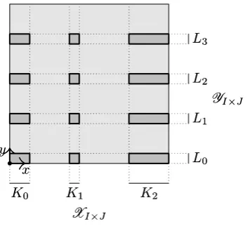
Figure 1. For a dyadic rectangle I×J ∈R, this gure depicts BI×J =XI×J×YI×J (the collection of the dark gray rectangles)
contained in the unit square (the light gray area). Here,XI×J = {K0, K1, K2}. The dyadic rectangles inKi×YI×J are connected
by dotted lines.
(v). Giveng ∈Hp(Hq)andε >0, we choose a nite subsetF ofR such that kg−P gkHp(Hq) ≤ε, where P : Hp(Hq)→ Hp(Hq) is the orthogonal projection
given by P f =P
R∈F hf,h|RR|ihR. Since the sets Bm, m ∈N, are pairwise disjoint
and F is nite, we can ndm0∈N such that Sm≥m0Bm
∩F =∅. Then, for
eachm≥m0 andγ∈Γ, we haveP∗fm= 0, and hence
|hMγg, fmi|=|hMγg,(I−P)∗fmi|=|hMγ(I−P)g, fmi| ≤ kMγk kg−P gkHp(Hq)kfmkHp(Hq)∗≤ε,
where we have used that Mγ commutes withP, and that kfmkHp(Hq)∗=|X|1−1/p|Y|1−1/q≤1
by (ii).
4.3. Embeddings and projections.
For each R ∈ R let XR,YR ⊂ D denote non-empty, nite collections of dyadic
intervals that dene the collection of dyadic rectanglesBR by
BR={K×L : K∈XR, L∈YR}, R∈R. (4.3)
Now (4.1) assumes the following form, if βR= 1 for eachR∈R:
bR(x, y) = X
K∈XR
hK(x) X
L∈YR
hL(y), R∈R; (4.4) see Figure 1.
Capon [3] discovered a condition for{BR:R∈R}which ensures that the block
basis {bR : R ∈ R} given by (4.4) is equivalent to the Haar system {hR : R ∈
R} in Hp(Hq), whenever 1 < p, q < ∞ (see Theorem 4.2). The local product
condition (P1)(P4) has its roots in Capon's seminal work [3]. We now introduce some notation. For R∈R we set
XR=[{K:K∈XR} and YR=
[
{L:L∈YR}. (4.5)
For each I0×J0∈Rwe consider the following unions
XI0 = [
{XI0×J :J ∈D}, YJ0= [
I
I0 I1
XI×J
XI0×J
XI1×J
K0
K
[image:9.595.133.473.93.220.2]x
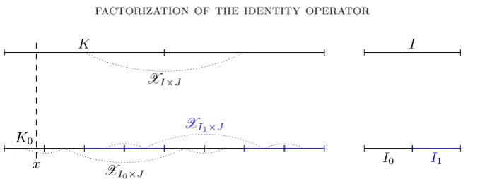
Figure 2. The gure depicts the collections XI×J, XI0×J,
XI1×J, with I0∪I1=I andI0∩I1 =∅,J ∈D. Givenx∈[0,1), the dashed vertical line connects the intervals K0 and K with x∈K0 ⊂K. By (P2) we haveXI0 ⊂XI, and in the gure (P4) is realized by |K∩XI0|
|K| = |XI0|
|XI|.
Clearly, for all I×J ∈R the following crucial inclusions hold true:
XI×J⊂XI and YI×J ⊂YJ. (4.7)
We say that {BI×J : I ×J ∈ R} given by (4.3) satises the local product
condition with constants CX, CY >0, if the following four properties (P1)(P4),
to be dened below, hold true.
(P1) For allR∈Rthe collectionBRconsists of pairwise disjoint dyadic rectangles,
and for allR0, R1∈Rwith R06=R1 we haveBR0∩BR1=∅.
(P2) For allI×J, I0×J0, I1×J1∈RwithI0∩I1=∅,I0∪I1⊂IandJ0∩J1=∅, J0∪J1⊂J we have
XI0∩XI1 =∅, XI0∪XI1 ⊂XI,
YJ0∩YJ1 =∅, YJ0∪YJ1 ⊂YJ.
(P3) For each R=I×J ∈R, we have
|I| ≤CX|XR|, |XI| ≤CX|I|, |J| ≤CY|YR|, |YJ| ≤CY|J|.
(P4) For allI0×J0, I×J ∈R withI0×J0⊂I×J and for everyK∈XI×J and L∈YI×J, we have
|K∩XI0|
|K| ≥C
−1 X
|XI0|
|XI| and
|L∩YJ0|
|L| ≥C
−1 Y
|YJ0|
|YJ|.
See Figure 2 for the collectionsXR,R∈R, and Figure 3 as well as Figure 4 for a
depiction ofXR andYR,R∈R.
Theorem 4.2 (Capon). Let 1≤p, q <∞. If the conditions (P1)(P3) are
satis-ed, then {bI×J : I×J ∈R} isC-equivalent to{hI×J : I×J ∈R} inHp(Hq),
where C depends only onCX andCY.
We emphasize that p or q may take the value 1 in the above theorem. By a duality argument, M. Capon [3] showed the equivalence stated in Theorem 4.2 implies that the orthogonal projectionP : Hp(Hq)→Hp(Hq)given by
P f = X
I×J∈R
hf, bI×Ji kbI×Jk22
bI×J (4.8)
is bounded on Hp(Hq), whenever1< p, q <∞. We point out that the parameters p = 1 or q = 1 are both excluded by the duality argument. Indeed, the duality argument of Capon shows that
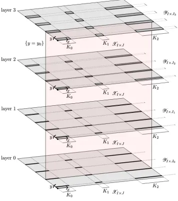
Figure 3. The dyadic rectangles I×J,I×J0 and I×J1 in R
are such thatJ0∪J1=J andJ0∩J1=∅. This gure depicts the
collections BI×J =XI×J×YI×J in the top layer, and BI×J0 =
XI×J0×YI×J0 andBI×J1 =XI×J1×YI×J1 in the bottom layer. Here, XI×J =XI0×J =XI1×J ={K0, K1, K2}. Each interval in
YI×J is split in two intervals, which are then placed into YI×J0 andYI×J1, respectively.
where the constants C(p, q, CX, CY) → ∞ in each of the cases p → 1, p → ∞, q→1or q→ ∞.
The next theorem is our rst major step towards proving Theorem 3.1. We show that the operatorP is bounded on Hp(Hq),1≤p, q <∞with an upper estimate
for the norm independent of p or q. Specically, Theorem 4.3 includes the cases p= 1or q= 1.
Theorem 4.3. Let 1≤p, q <∞, let{BR : R∈R} be a pairwise disjoint family
which satises the local product condition (P1)(P4) with constants CX and CY,
and letβ = (βQ:Q∈S
R∈RBR)be a family of scalars such that M := sup
Q
|βQ|<∞.
Then the operators Bβ, Aβ :Hp(Hq)→Hp(Hq)given by
Bβf = X
R∈R hf, hRi
khRk2 2
b(β)R and Aβf =
X
R∈R
hf, b(β)R i kbRk2
2 hR
satisfy the estimates
kBβfkHp(Hq)≤M CX1/pCY1/qkfkHp(Hq), f ∈Hp(Hq),
kAβfkHp(Hq)≤M CX3+1/pCY3+1/qkfkHp(Hq), f ∈Hp(Hq).
(4.9)
If we additionally assume that
m:= inf
Figure 4. In the gure, XI×Jj = {K0, K1, K2}, 0 ≤ j ≤ 3,
whereasYI×Jj changes with each layer0≤j≤3. Fory0 ∈[0,1),
the light red vertical plane connects the lines ` = {(x, y0) : x ∈
[0,1)}in the four layers depicted in the gure.
and if we dene the vector of scalarsγ= γQ :Q∈S
R∈RBRbyβQγQ = 1, then
the diagram
Hp(Hq) IHp(Hq) //
Bβ %%
Hp(Hq)
Hp(Hq) Aγ
9
9
(4.10)
is commutative, and the operatorAγ satises the estimatekAγk ≤m−1C3+1/p
X C
3+1/q
Y .
Moreover, the compositionPβ,γ =BβAγ is the projectionPβ,γ :Hp(Hq)→Hp(Hq)
given by
Pβ,γ(f) = X
R∈R
hf, b(γ)R i kbRk2
Consequently, the range of Bβ is complemented (by Pβ,γ), and Bβ is an
isomor-phism onto its range. Finally, ifβQ=γQ= 1for eachQ, thenPβ,γ coincides with
the orthogonal projection P dened by (4.8).
Before we proceed with the proof, we record some simple facts.
Lemma 4.4. Let BR = XR×YR ⊂ R, R ∈ R satisfy the conditions (P1)
and (P3). Then
CX−1CY−1|R| ≤ kbRk22≤CXCY|R|, R∈R.
Proof. Let R∈R be xed. By condition (P1) and (4.3), the collectionsXR and
YR each consist of pairwise disjoint dyadic intervals, thus, Lemma 4.1 (i) yields kbRk22=|XR||YR|.
By (P3) and (4.7) we obtain
CX−1CY−1|R| ≤ |XR||YR| ≤CXCY|R|. Below we use Minkowski's inequality in various function spaces. For ease of reference, we include it in the form that we need it.
Lemma 4.5. Let(Ω, µ)be a probability space.
(i) Let1≤r <∞ and letgk∈Lr(Ω) be real valued. Then
Z
Ω
X
k gk2
r/2
dµ≥ X k
Z
Ω
gkdµ2r/2
.
(ii) Let 1≤r, s <∞ and letgk,`∈Ls(Ω) be real valued. Then
Z Ω X k X ` gk,`2
s/2r/s
dµ≥
X k X ` Z Ω
gk,`dµ2s/2
r/s
.
Proof. First, we apply Minkowski's inequality (see e.g. [6, Corollary 5.4.2], [9, The-orem 202]) to the integral and the sum over`:
X k X ` Z Ω
gk,`dµ2s/2
1/s ≤ X k Z Ω X ` g2k,`
1/2
dµs
1/s
.
Secondly, applying Minkowski's inequality to the integral and the sum overkyields
X k Z Ω X ` g2k,`
1/2
dµs
1/s ≤ Z Ω X k X ` gk,`2
s/21/s
dµ.
Finally, we obtain (ii) by Hölder's inequality.
The assertion (i) follows from (ii) by puttings= 2. Lemma 4.6. Assume that (ZI :I ∈D) satises the following condition: For all
I, I0, I1∈D withI0∩I1=∅,I0∪I1⊂I we have that ZI0∩ZI1 =∅ and ZI0∪ZI1⊂ZI. Let 0< r <∞,N0∈NandcI ≥0 and dene
f(z) = X
I∈DN0
cI1ZI(z)
r
.
Then
e
cI = X
E⊃I
cEr− X E)I
cEr
satises ecI ≥0 and we obtain the identity
f(z) = X
I∈DN0 e
Proof. Observe that by telescoping and the tree structure of the sets (ZI :I∈D) we have that
X
I∈DN0
cI1ZI(z)
r
= X
I∈DN0 e
cI1ZI(z).
The fact thatecI ≥0 is self-evident.
Proof of Theorem 4.3. The proof will be split into three parts. In the rst part, we will give the estimate forBβ, and in the second part, we will establish the estimate
forAβ.
Part 1: The estimate forBβ. We emphasize that our proof of the estimate for Bβ only uses the conditions (P1)(P3); specically, we do not use (P4).
ForN0∈Nwe dene the collections of indices
RN0 ={I0×J0∈R : I0, J0∈DN0} (4.11a) and
RN0 ={I0×J0∈R : I0, J0∈DN0}. (4.11b) Let us assume that
f = X
R∈RN0
aRhR.
Then by (P1) and (4.3) we nd that
kBβfkpHp(Hq)=
Z 1
0
Z 1
0
X
R∈RN0
|aR|2 X Q∈BR
|βQ|21Q(x, y)
q/2
dy
p/q
dx.
Recall that |βI×J| ≤ M and that by (4.7) 1XI×J(x)1YI×J(y) ≤1XI(x)1YJ(y), so
we note
kBβfkpHp(Hq)≤M pZ 1 0 Z 1 0 X
I×J∈RN0
|aI×J|21XI(x)1YJ(y)
q/2
dy
p/q
dx.
(4.12) If we dene cJ(x) =P
I∈DN0|aI×J|
21
XI(x), (4.12) reads
kBβfkpHp(Hq)≤M pZ 1 0 Z 1 0 X
J∈DN0
cJ(x)1YJ(y)
q/2
dy
p/q
dx. (4.13)
Lemma 4.6 yields the following identity for the inner integrand of (4.13):
X
J∈DN0
cJ(x)1YJ(y)
q/2
= X
J∈DN0
ecJ(x)1YJ(y), (4.14)
where ecJ(x) = P
J1⊃JcJ1(x)
q/2
− P
J1)JcJ1(x)
q/2
≥ 0. Integrating (4.14)
with respect to y and using that|YJ| ≤CY|J| by (P3), we have
Z 1
0
X
J∈DN0
cJ(x)1YJ(y)
q/2
dy≤CY X J∈DN0
e
cJ(x)|J|.
Combining the latter estimate with (4.13) yields
kBβfkpHp(Hq)≤M pCp/q
Y
Z 1
0
X
J∈DN0 e
cJ(x)|J|
p/q
It remains to estimateR1
0
P
J∈DN0ecJ(x)|J|
p/q
dxfrom above by a constant
mul-tiple of kfkpHp(Hq). Note that
X
J1⊃J
cJ1(x)
q/2
= X
I∈DN0
dI,J1XI(x)
q/2
, wheredI,J = X
J1⊃J
|aI×J1|
2,
X
J1)J
cJ1(x)
q/2
= X
I∈DN0
eI,J1XI(x)
q/2
, whereeI,J = X
J1)J
|aI×J1|
2,
and thatecJ(x)was dened as the dierence between the two quantities, above. By Lemma 4.6, we obtain
X
I∈DN0
dI,J1XI(x)
q/2
= X
I∈DN0 e
dI,J1XI(x),
X
I∈DN0
eI,J1XI(x)
q/2
= X
I∈DN0 e
eI,J1XI(x),
where
e
dI,J = X
I1⊃I
dI1,J
q/2
− X I1)I
dI1,J
q/2
≥0,
e
eI,J = X
I1⊃I
eI1,J
q/2
− X I1)I
eI1,J
q/2
≥0.
Summing up, in between (4.15) and here, we have shown that
kBβfkpHp(Hq)≤M pCp/q
Y
Z 1
0
X
I∈DN0
fI1XI(x)
p/q
dx, (4.16)
where fI =P
J∈DN0|J|(dI,Je −eeI,J).
It is important to show that fI ≥ 0, for all I ∈ DN0. To this end, note the identity
e
dI,J−eeI,J = X
I1⊃I
J1⊃J
|aI1×J1|
2q/2− X
I1)I J1⊃J
|aI1×J1|
2q/2
− X I1⊃I
J1)J
|aI1×J1|
2q/2+ X
I1)I
J1)J
|aI1×J1|
2q/2.
Let J0 ∈DN0, then grouping together the rst with the third term as well as the
second with the fourth, and summing the latter identity over J⊃J0 yields
X
J⊃J0 e
dI,J −eeI,J = X
I1⊃I
J1⊃J0
|aI1×J1|
2q/2− X
I1)I
J1⊃J0
|aI1×J1|
2q/2≥0.
Since we have
fI = X
J0∈DN0
|J0| X J⊃J0
(dI,Je −eeI,J),
we showed thatfI ≥0.
A nal application of Lemma 4.6 gives
Z 1
0
X
I∈DN0
fI1XI(x)
p/q
dx=
Z 1
0
X
I∈DN0 e
fI1XI(x) dx=
X
I∈DN0 e
where fIe = PI 1⊃IfI
p/q
− P
I1)IfI
p/q
≥0. Using (P3) in the above identity
and combining it with (4.16) yields
kBβfkpHp(Hq)≤CXM pCp/q
Y
X
I∈DN0 e
fI|I|.
Finally, we remark that
kfkpHp(Hq)=
X
I∈DN0 e
fI|I|.
To see this, it suces to apply Lemma 4.6 as above.
Part 2: The estimate forAβ. LetN0∈N, and dene the collections of building
blocks BN0 andB
N0 by
BN0={K0×L0∈BI0×J0 : I0×J0∈RN0} and
BN0 ={K×L∈B
I×J : I×J ∈RN0},
where RN0 and R
N0 are dened in (4.11). Taking into account that the bi-parameter Haar system is a1-unconditional basis ofHp(Hq), it suces to consider
only thosef that can be written as follows:
f = X
K×L∈BN0
aK×LhK×L.
We will now estimate kAβfkpHp(Hq). To this end, note that by the denitions of Aβ and the norm inHp(Hq)we have
kAβfkpHp(Hq)=
Z 1
0
Z 1
0
X
R∈RN0
|hf, b(β)R i|2 kbRk4
2
1R(x, y)
q/2
dy
p/q
dx.
SinceDN0 is a partition of the unit interval, we obtain that
kAβfkpHp(Hq)=
X
I0∈DN0 Z
I0
X
J0∈DN0 Z
J0
X
R∈RN0
|hf, b(β)R i|2 kbRk4
2
1R(x, y)
q/2
dy
p/q
dx.
Recall that |βQ| ≤M, note that for I0, J0 ∈DN0 and R ∈ R
N0 as in the above sums, 1R(x, y) = 1exactly whenR⊃I0×J0, and apply Lemma 4.4 to obtain
kAβfkpHp(Hq)
≤MpCp XC
p Y
X
I0∈DN0
|I0|
X
J0∈DN0
|J0| X R∈RN0
R⊃I0×J0
X
Q∈BR
|aQ||Q| |R|
2q/2p/q
. (4.17)
We continue by proving a lower bound forkfkpHp(Hq). Set
wR= X
Q∈BR
|aQ|hQ, R∈RN0,
and observe that by (P1) we have
kfkpHp(Hq)=
Z 1
0
Z 1
0
X
R∈RN0
wR2(x, y)
q/2
dy
p/q
dx.
By (P2) the collections {XI0 :I0 ∈DN0}and {YJ0 :J0∈DN0} are each pairwise disjoint, thus we obtain
kfkpHp(Hq)≥
X
I0∈DN0 Z
XI0
X
J0∈DN0
|YJ0| Z
YJ0
X
R∈RN0
w2R(x, y)
q/2 dy
|YJ0|
p/q
For xed I0, J0∈DN0,x∈XI0,y∈YJ0 andR∈R
N0, we have by (4.7) and (P2) that wR(x, y) 6= 0 implies R ⊃ I0×J0, so we obtain from the latter estimate
together with (P3) the following lower estimate forCYp/qkfkpHp(Hq):
X
I0∈DN0 Z
XI0
X
J0∈DN0
|J0|
Z
YJ0
X
R⊃I0×J0
w2 R(x, y)
q/2 dy
|YJ0|
p/q
dx. (4.18)
WithI0, J0∈DN0 xed, we now prepare for the application of Lemma 4.5 to the inner integral of the above estimate. We use the following specication. We put Ω =YJ0, dµ=
dy
|YJ0|, andr=q. In view of (i) of Lemma 4.5 we obtain that Z
YJ0
X
R⊃I0×J0
wR2(x, y)
q/2 dy
|YJ0|
≥ X
R⊃I0×J0
Z
YJ0
|wR(x, y)| dy |YJ0|
2q/2
.
(4.19) By (P1) we have|wR(x, y)|=P
K×L∈BR|aK×L|1K(x)1L(y), hence by (P4) and (P3)
Z
YJ0
|wR(x, y)| dy |YJ0|
= X
K×L∈BR |aK×L|
|L∩YJ0|
|YJ0|
1K(x)
≥CY−2
X
K×L∈BR
|aK×L||L||J|1K(x)
for allR∈RN0 withR=I×J ⊃I0×J0. Combining the latter estimate with (4.19) and (4.18) we obtain the following lower estimate for CY2p+p/qkfkpHp(Hq):
X
I0∈DN0
|XI0| Z
XI0
X
J0∈DN0
|J0| X R⊃I0×J0
vR2(x)
q/2p/q dx
|XI0|
, (4.20)
where we put vR(x) =P
K×L∈BR |aK×|JL|||L|1K(x), if R =I×J. With I0 ∈ DN0 xed, we now prepare for the application of Lemma 4.5 to obtain a lower bound for the following term:
Z
XI0
X
J0∈DN0
|J0| X R⊃I0×J0
vR2(x)
q/2p/q dx
|XI0|
. (4.21)
To this end, we use the following specication. We put Ω =XI0, dµ= dx
|XI0|, and
r=p,s=q. Invoking (ii) of Lemma 4.5, we nd that (4.21) is bounded from below
by
X
J0∈DN0
|J0| X R⊃I0×J0
Z
XI0
vR(x) dx
|XI0|
2q/2p/q
. (4.22)
Recall that we denedvR(x) =P
K×L∈BR|aK×|JL|||L|1K(x), ifR=I×J. By (P4)
and (P3) we estimate Z
XI0
vR(x) dx
|XI0|
= X
K×L∈BR
|aK×L||L|
|J|
|K∩XI0|
|XI0|
≥CX−2 X Q∈BR
for all R = I ×J ∈ RN0 with R ⊃ I0×J0. Combining the latter estimate
with (4.22), (4.21), and (4.20), we obtain the following lower estimate forCX2pCY2p+p/qkfkpHp(Hq):
X
I0∈DN0
|XI0|
X
J0∈DN0
|J0| X R⊃I0×J0
X
Q∈BR
|aQ||Q| |R|
2q/2p/q
.
Finally, by (P3) the latter estimate yields
CX2p+1CY2p+p/qkfkpHp(Hq)≥
X
I0∈DN0
|I0|
X
J0∈DN0
|J0| X R⊃I0×J0
X
Q∈BR
|aQ||Q| |R|
2q/2p/q
. (4.23)
Direct comparison with (4.17) gives
kAβfkHp(Hq)≤M CX3+1/pCY3+1/qkfkHp(Hq).
Part 3: Conclusion of the proof. If additionally, we assume that m := infQ|βQ| > 0, Part 2 implies that Aγ is bounded by m−1CX3+1/pC
3+1/q
Y . The
commutativity of the diagram (4.10) follows from the fact that βQγQ = 1. 4.4. A linear order onRRR and Capon's local product condition.
In Section 5, we will iteratively construct collections of dyadic rectanglesBR⊂R, R ∈ R satisfying Capon's local product condition. This will be accomplished
by organizing the dyadic rectangles according to the linear order C dened in the present section, below. The other purpose of this section is to introduce the auxiliary condition (R1)(R6) and to show that it implies Capon's local product condition (P1)(P4).
First, we dene the bijective function ON2 0 :N
2
0→N0 by
ON20(m, n) = (
n2+m, ifm < n, m2+m+n, ifm≥n.
To see thatON2
0 is bijective consider that for eachk∈N:
. ON2
0(0,0) = 0,
. m 7→ ON2
0(m, k) maps {0, . . . , k−1} bijectively onto {k
2, . . . , k2+k−1}
and preserves the natural order on N0, . ON2
0(k,0) =ON20(k−1, k) + 1,
. n 7→ON2
0(k, n) maps {0, . . . , k} bijectively onto{k
2+k, . . . , k2+ 2k} and
preserves the natural order onN0, . ON2
0(0, k+ 1) =ON20(k, k) + 1. See Figure 5 for a depiction of ON2
0.
Now, let <` denote the lexicographic order on R3. For two dyadic rectangles Ik×Jk∈R with|Ik|= 2−mk,|Jk|= 2−nk,k= 0,1, we deneI0×J0CI1×J1 if
and only if
ON20(m0, n0),infI0,infJ0
<` ON2
0(m1, n1),infI1,infJ1
.
Associated to the linear ordering C is the bijective index function OC :R →N0
dened by
OC(R0)<OC(R1)⇔R0CR1, R0, R1∈R.
The geometry of a dyadic rectangle is linked to its index by the estimate
(0,0)
(0,1)
(1,0)
(1,1)
(0,2) (1,2)
(2,0)
(2,1)
(2,2)
(0,3) (1,3) (2,3)
(3,0)
(3,1)
(3,2)
[image:18.595.198.399.121.311.2](3,3)
Figure 5. This gure depicts the order of the rst 16 pairs inN20
with respect to the map ON20.
0
1 2
3 4
5 6
7 8
9 10 11 12 13 14
15 16
17 18
19 20
21 22 23 24
25 26 27 28
29 30 31 32
33 34 35 36
37 38 39 40
41 42 43 44
45 46 47 48
Figure 6. The rst49rectangles and their indicesOC.
and hence,
1
(1 +√i)2 ≤ |I| |J|, i=OC(I×J). (4.25)
The index of a dyadic rectangle and its predecessors are related by e
I×JCI×J, forI6= [0,1) and I×JeCI×J, forJ6= [0,1), (4.26) where we recall that for I6= [0,1),Ieis the unique dyadic interval satisfyingIe⊃I and |I|e = 2|I|. See Figure 6 for a picture ofOC.
For a dyadic interval I, we write I` and Ir for the dyadic intervals which are
the left and right halves of I, respectively. In the following denition, we use the
notation introduced in (4.5), so that for a collectionXR(respectively,YR) of dyadic
[image:18.595.211.386.362.542.2]Denition 4.7. Let A =R or A ={R ∈ R : RER0} for some R0 ∈ R. We
say that{BR:R∈A}satises the auxiliary condition (R1)(R6) if the following
properties hold true.
(R1) For each R∈A, there are non-negative integersµ(R), ν(R)and non-empty sets XR ⊂Dµ(R)and YR⊂Dν(R) such thatBR ={K×L:K∈XR, L∈
YR}.
(R2) µ([0,1)×[0,1)) =ν([0,1)×[0,1)) = 0andX[0,1)×[0,1)=Y[0,1)×[0,1)={[0,1)}.
(R3) For eachI∈D\ {[0,1)}withR=I×[0,1)∈A
XI×[0,1)=
(S{K`:K∈Dκ(R), K⊂X
e
I×[0,1)} if I=Ie`, S
{Kr:K∈Dκ(R), K⊂X
e
I×[0,1)} if I=Ier, whereκ(R) = max{µ(S) :SC[0,|I|)×[0,1)};
(R4) IfR=I×J ∈A with|I|<|J|, then
µ(R)>max{µ(S) :SCR},
XR =XI×[0,1), andYR=YI0×J, whereI0 ∈D is the unique dyadic interval
such thatI0⊃I and|I0|=|J|.
(R5) For J ∈D\ {[0,1)}withR= [0,1)×J∈A
Y[0,1)×J =
(S
{L`:L∈Dλ(R), L⊂Y
[0,1)×Je} if J =Je
`,
S{Lr:L∈Dλ(R), L⊂Y
[0,1)×Je} if J =Je
r,
whereλ(R) = max{ν(S) :SC[0,1)×[0,|J|)}.
(R6) IfR=I×J ∈A \ {[0,1)×[0,1)}with|I| ≥ |J|, then ν(R)>max{ν(S) :SCR},
YR=Y[0,1)×J, and XR=XI×J0, where J0 ∈D is the unique dyadic interval
such thatJ0⊃J and|J0|= 2|I|ifI6= [0,1), andJ0= [0,1)ifI= [0,1).
Remark 4.8. Let{BR:R∈R} be a collection such that each of the nite
sub-collections {BR : RER0}, R0 ∈ R, satises the auxiliary condition (R1)(R6).
Then it is easy to see that {BR : R ∈ R} itself satises the auxiliary condition
(R1)(R6).
Lemma 4.9. Let {BR :R∈R} satisfy the auxiliary condition (R1)(R6). Then {BR:R∈R} satises the local product condition (P1)(P4) with constantsCX = CY = 1.
Proof. The usual linear order ≺on dyadic intervals is given byI1≺I0 if and only
if either |I1| > |I0| or |I1| = |I0| and minI1 < minI0. The proof uses induction
with respect to the linear orders≺andC.
Verification of (P1). For eachR∈R,XRconsists of pairwise disjoint intervals
because XR is contained inDµ(R). Similarly,YR⊂Dν(R) and consists of pairwise
disjoint intervals, and therefore the rectangles in BR are pairwise disjoint.
Now suppose that R0, R1∈Rare distinct. By relabelling them if necessary, we
may suppose that R1CR0, whereR0=I0×J0 6= [0,1)×[0,1). To establish the
disjointness ofBR0 andBR1, we must show that eitherXR0 andXR1 are disjoint or YR0 andYR1 are disjoint. If|I0|<|J0|, then (R4) implies thatµ(R0)> µ(R1), so that XR0∩XR1 ⊂Dµ(R0)∩Dµ(R1)=∅. Otherwise |I0| ≥ |J0|, in which case a similar argument based on (R6) shows thatYR0∩YR1=∅.
Verification of (P2). We begin by observing that (R4) and (R6) imply that the setsXR,YR,XI, andYJ dened in (4.5)(4.6) are given by
Since the order ≺ is linear, and the set D is countable and has a minimum
el-ement [0,1) with respect to ≺, we may use induction on I0 ∈ D to prove the
following two statements:
(a) XI0×[0,1)∩XI1×[0,1) = ∅ and Y[0,1)×I0 ∩Y[0,1)×I1 = ∅ for each I1 ∈ D with
I1≺I0and I0∩I1=∅;
(b) XI0×[0,1)⊂XI1×[0,1)andY[0,1)×I0 ⊂Y[0,1)×I1 for eachI1∈D withI0⊂I1. The statements (a) and (b) above together with (4.27) imply (P2). The start of the induction is easy. Indeed, suppose that I0= [0,1). Then noI1satisesI1≺[0,1),
so that (a) is vacuous, while (b) holds trivially becauseI1= [0,1)is the only dyadic interval which contains [0,1).
Now letI0∈D\ {[0,1)}, and assume inductively that (a)(b) have been
estab-lished for each I00 ≺I0 (that is, (a)(b) hold wheneverI0 is replaced withI00). We
shall prove the statements concerningXI0×[0,1); the proofs forY[0,1)×I0 are similar, requiring only minor adjustments of the notation.
To verify (a), suppose thatI1∈D satisesI1≺I0andI0∩I1=∅. Then either I1∩I0e =∅, orI1 = (eI0)` andI0 = (eI0)r. (Note that because I1 ≺I0, we cannot have I1 = (eI0)r and I0 = (eI0)`.) In the rst case, since I1 ≺I0 and
e
I0 ≺I0, the
induction hypothesis implies that XIe0×[0,1)∩XI1×[0,1)=∅, from which the result follows because XI0×[0,1)⊂XIe0×[0,1)by (R3).
In the second case, we observe thatI0e =I1e and|I0|=|I1|, so thatκ(I0×[0,1)) =
κ(I1×[0,1)). This implies thatXI0×[0,1)andXI1×[0,1)are disjoint becauseXI0×[0,1) is the disjoint union of the right halves of the intervals K ∈ Dκ(I0×[0,1)) with
K ⊂XIe0×[0,1), while XI1×[0,1) is the disjoint union of the left halves of the same intervals.
Next, to prove (b), suppose that I1 ∈D with I0 ⊂I1. The inclusion is obvious
ifI0=I1, so we may suppose thatI0(I1. Then we haveI0e ⊂I1, so the induction hypothesis implies that XIe0×[0,1) ⊂XI1×[0,1). Hence the statement follows from the fact thatXI0×[0,1)⊂XIe0×[0,1).
Verification of (P3). The proofs of (P3) and (P4) both rely on the following two identities:
|K∩XI×[0,1)|=
|K∩XeI×[0,1)|
2 and |L∩Y[0,1)×J|=
|L∩Y[0,1)×Je|
2 , (4.28) valid forI, J ∈D\ {[0,1)}, K∈Dκ(I×[0,1)), andL∈Dλ([0,1)×J).
We shall establish the rst of these identities; again, the proof of the other requires only notational changes. For I ∈ D \ {[0,1)} and K ∈ Dκ(I×[0,1)), set VI(K) ={K0∈Dκ(I×[0,1)):K0⊂K∩XIe×[0,1)}. We claim that
K∩XIe×[0,1)=[VI(K) and K∩XI×[0,1)=
(S
{K`
0:K0∈VI(K)} ifI=Ie` S
{Kr
0 :K0∈VI(K)} ifI=Ier. (4.29) Indeed, the inclusionS
VI(K)⊂K∩XIe×[0,1)is clear from the denition ofVI(K). Conversely, for each x ∈ K∩XIe×[0,1), there is a (necessarily unique) interval K0 ∈ XIe×[0,1) such that x ∈ K0. We have µ(eI×[0,1)) ≤κ(I×[0,1)) because
e
I×[0,1)C[0,|I|)×[0,1), so we can ndK1∈Dκ(I×[0,1)) such thatx∈K1⊂K0.
The setsK1andKare not disjoint as they both containx; combined with the fact
that |K1| ≤ |K|, this shows thatK1⊂K. Moreover, we haveK1⊂K0⊂XIe×[0,1),
so thatK1∈VI(K), and hencex∈K1⊂SVI(K).
Moving on to the second part of (4.29), we obtain the inclusion⊃directly from
that x ∈ K and either x ∈ K`
0 or x ∈ K0r (depending on whether I = (Ie)` or
I= (eI)r) for someK0∈D
κ(I×[0,1)) withK0⊂XIe×[0,1). In both cases, we see that
K∩K06=∅and|K0| ≤ |K|, so thatK0 ⊂K, and henceK0∈VI(K), from which
the inclusion follows.
The rst equation in (4.28) is immediate from (4.29) because VI(K)consists of
disjoint sets and |K`
0|=|K0r|=|K0|/2.
We can now easily establish (P3) withCX =CY = 1. By (4.27), we must show
that
|XI×[0,1)|=|I| and |Y[0,1)×I|=|I|, I∈D. (4.30)
We do so by induction on I. The start of the induction, whereI = [0,1), follows
immediately from the fact thatX[0,1)×[0,1)=Y[0,1)×[0,1)= [0,1)by (R2).
Now letI∈D\ {[0,1)}, and assume inductively that the result is true for each I0 ≺I. Using (4.28) withK=L= [0,1), we obtain that|XI
×[0,1)|=|XIe×[0,1)|/2 =
|I|/e 2 =|I|because Ie≺I and likewise|Y[0,1)×I|=|I|.
Verification of (P4). We shall prove that, for eachR0=I0×J0andR=I×J
in R withR0⊂R, |K∩XI0×[0,1)|
|I0| = |K|
|I| and
|L∩Y[0,1)×J0|
|J0| = |L|
|J|, K∈XR, L∈YR.
(4.31) By (4.27) and (4.30), this will verify (P4) with CX =CY = 1.
The proof of (4.31) is by induction on R0. The start of the induction is trivial
because the onlyR∈R that containsR0= [0,1)×[0,1)isR0 itself.
Now let R0∈R\ {[0,1)×[0,1)}, and assume inductively that (4.31) has been
veried for each R0
0CR0. This time, we shall focus on the proof of the second
identity in (4.31); the proof of the rst identity is similar, but formally slightly easier due to the lack of symmetry between conditions (R4) and (R6): when|I|=|J|, we
re-use an existing set asXRand dene a new setYR.
Suppose that R =I×J ∈ R with R0 ⊂R, and letL ∈ YR. If J0 = J, then L⊂Y[0,1)×J0, and the identity is immediate. Hence we may suppose thatJ0(J. Moreover, we may suppose that|I| ≥ |J|. Indeed, if not, then by (R4)YR=YI0×J,
where I0 ∈D satises I0 ⊃I and |I0| =|J|, so that we may replaceI with I0 to
obtain that|I| ≥ |J|.
Then we have|J0|<|J|= min{|I|,|J|}, so that RC[0,1)×[0,|J0|), and hence λ([0,1)×J0)≥ν(R); thusL∈YR⊂Dν(R)⊂Dλ([0,1)×J0), so that (4.28) shows that |L∩Y[0,1)×J0|=|L∩Y[0,1)×Je0|/2. NowR
0
0=I0×J0e satisesR00 CR0andR00⊂R, and therefore the induction hypothesis implies that |L∩Y[0,1)×Je0|/|J0e|=|L|/|J|. Hence the conclusion follows because|J0e|= 2|J0|. Having obtained Theorem 4.3 and Lemma 4.9, we are nally prepared to prove Theorem 3.1.
5. Proof of Theorem 3.1
Here, we prove that the identity operator onHp(Hq)factors through any operator T : Hp(Hq) → Hp(Hq) having large diagonal with respect to the bi-parameter
Haar system (see Theorem 3.1). The basic pattern of our argument below is the following: we carefully construct {BR:R ∈R} satisfying the auxiliary condition
(R1)(R6) (see Section 4). Moreover, these collections are chosen in such a way that we are able to nd signsεQ∈ {±1},Q∈S
R∈RBR, for which the block basis b(ε)R =P
Q∈BRεQhQ,R∈R has the following properties: |hT b(ε)R1, b
(ε)
the precise sense of (5.6a) below whenever R1, R2∈R are distinct, and
|hT b(ε)R , b(ε)R i| ≥δkbR(ε)k22, R∈R.
Thereafter we apply the two main results of the preceding section, Theorem 4.3 and Lemma 4.9, and nally we construct a factorization of the identity operator throughT.
Proof of Theorem 3.1. Let1≤p, q <∞andδ >0, and letT :Hp(Hq)→Hp(Hq)
be an operator such that
|hT hR, hRi| ≥δ|R|, R∈R. (5.1)
We deneγ= (γR:R∈R)by
γR= hT hR, hRi
|hT hR, hRi|, R∈R.
Recall that in (4.2) we dened the Haar multiplier Mγ which satises kMγk = 1,
andh(T Mγ)hR, hRi ≥δ|R|. Thereby, replacingT withT Mγ, it suces to consider
the special case where
hT hR, hRi ≥δ|R|, R∈R. (5.2)
Overview. Let 0 < η ≤ 1. The main part of the proof consists of choosing
collections of dyadic rectangles BR, R∈R and suitable signsε= (εQ)such that b(ε)R =P
Q∈BRεQhQ satises the following:
. The closed linear span of {b(ε)R :R ∈R} is complemented and isomorphic
to Hp(Hq).
. There is an operator U :Hp(Hq)→Hp(Hq)given by U(f) = X
R∈R
hf, b(ε)R i hT b(ε)R , b(ε)R ib
(ε) R .
. For every nite linear combination g=P
R∈RλRb(ε)R we have kU T g−gkHp(Hq)≤
η
2kgkHp(Hq). Preparation. Given R=I×J ∈R we write
T hR=αRhR+rR, (5.3a)
where
αR= hT hR, hRi
|R| and rR=
X
S6=R
hT hR, hSi
|S| hS. (5.3b)
We note the estimates
δ≤αR≤ kTk and krRkHp(Hq)≤2kTk|I|1/p|J|1/q. (5.4)
Inductive construction ofb(ε)R . We will now inductively dene the block basis {b(ε)R : R∈R}. For xedR∈R, the block basis elementb(ε)R is determined by a
collection of dyadic rectangles BR⊂Rand a suitable choice of signsε= (εQ)and
is of the following form:
b(ε)R = X
Q∈BR
εQhQ. (5.5)
From now on, we systematically use the following rule: whenever OC(R) =i we
set
Bi =BR, b(ε)i =b (ε)
We will construct collections{Bi:i∈N0}satisfying the auxiliary condition (R1)
(R6) and choose signs ε= (εQ)such that
i−1
X
j=0
|hT b(ε)j , b(ε)i i|+|hb(ε)i , T∗b(ε)j i| ≤ηδ4−i−2, i∈
N, (5.6a) |hT b(ε)i , b(ε)i i| ≥δkbi(ε)k22, i∈N0. (5.6b)
The induction begins by putting
B0={[0,1)×[0,1)} and b(ε)0 =h[0,1)×[0,1). (5.7)
Consequently,X[0,1)×[0,1)=Y[0,1)×[0,1)={[0,1)}andµ([0,1)×[0,1)) = 0,ν([0,1)×
[0,1)) = 0. Obviously,{B0}satises (R1)(R6).
Leti0∈N. At this stage we assume that
. {Bj : 0≤j≤i0−1} satises the auxiliary condition (R1)(R6).
. the block basis {b(ε)j : 0 ≤ j ≤ i0−1} given by (5.5) satises (5.6) (for
0≤i≤i0−1).
Now, we turn to the construction of Bi0 andεQ, whereQ∈Bi0. In the rst step we will nd Bi0 in (5.20), and only then we will choose the signs εQ, Q ∈ Bi0 in (5.23). The collectionBi0 and the signs εQ,Q∈Bi0 then determineb
(ε) i0 . Construction of Bi0. Let I0×J0 ∈ R be such that OC(I0×J0) = i0. We distinguish between the four cases
|I0|<|J0|, J0= [0,1), |I0|<|J0|, J06= [0,1),
and
|I0| ≥ |J0|, I0= [0,1), |I0| ≥ |J0|, I06= [0,1).
Case 1: |I0|<|J0|. Here, we will construct the collectionBI0×J0, for which the index rectangle I0×J0 is below the diagonal.
First, we dene
ν(I0×J0) =ν(I00 ×J0) and YI0×J0 =YI00×J0, (5.8) where I0
0∈D is the unique interval such thatI00 ⊃I0 and |I00|=|J0|. We remark
that µ(I0×J0)will be dened at the end of the proof in (5.21a). Case 1.a: J0= [0,1). Here, we know thatI06= [0,1). Recall
that I0e denotes the dyadic predecessor of I0, and note that
BIe0×[0,1)has already been dened. The collections indexed by
the black rectangles have already been constructed. Here, we determine the collections for the gray rectangles. The white ones will be treated later.
Note that [0,|I0|)×[0,1)EI0×[0,1), and dene the integerκ(I0×[0,1))by
κ(I0×[0,1)) = max{µ(Q) :QC[0,|I0|)×[0,1)}.
Recall that for a dyadic interval K0 we denote its left half by K`
0 and its right
half by Kr
0. Following the basic construction of Gamlen-Gaudet [5], we proceed
as follows. The set XIe0×[0,1) has already been dened in a previous step of the
construction. Now we put
XI0×[0,1)= (
S{K`
0:K0∈Dκ(I0×[0,1)), K0⊂XIe0×[0,1)} if I0=I0e
` ,
S{Kr
0 :K0∈Dκ(I0×[0,1)), K0⊂XIe0×[0,1)} if I0=I0e
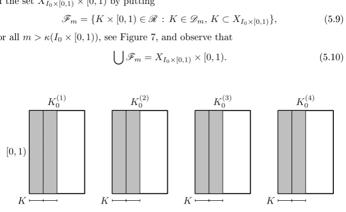
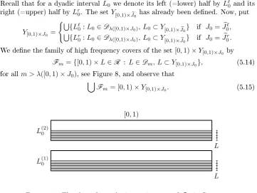
To nish the construction in Case 1.a, we dene the family of high frequency covers of the set XI0×[0,1)×[0,1)by putting
Fm={K×[0,1)∈R : K∈Dm, K⊂XI0×[0,1)}, (5.9) for allm > κ(I0×[0,1)), see Figure 7, and observe that
[
Fm=XI0×[0,1)×[0,1). (5.10)
[0,1)
K0(1)
K
K0(2)
K
K0(3)
K
K0(4)
[image:24.595.124.479.135.352.2]K
Figure 7. The above gure depicts an instance ofFmin Case 1.a. K0(k) is a dyadic interval such that K
(k)
0 ×[0,1) ∈BIe0×[0,1), and
K is a dyadic interval such thatK×[0,1)∈Fm.
Case 1.b: J0 6= [0,1). The collections indexed by the black
rectangles have already been constructed. Here, we determine the collections for the gray rectangles. The white ones will be treated later.
By our induction hypothesis, {BI×J : OC(I×J) ≤i0−1} satises (R1)(R6).
Note that the set XI0×[0,1) is already dened. To conclude the construction in Case 1.b, we dene the high frequency covers ofXI0×[0,1)×YI0×J0 by
Fm={K×L0∈R : K∈Dm, K⊂XI0×[0,1), L0∈YI0×J0}, (5.11) form > µ(I0×J0e).
Case 2: |I0| ≥ |J0|. In this case, we will construct the collectionBI0×J0, for which the index rectangleI0×J0 is on or above the diagonal.
First, we set
µ(I0×J0) =µ(I0×J00) and XI0×J0 =XI0×J00, (5.12) where J00 ∈D is the unique dyadic interval such that J00 ⊃J0 and |J00| = 2|I0| if I06= [0,1), andJ00 = [0,1) ifI0= [0,1). We remark thatν(I0×J0)will be dened
at the end of the proof in (5.21b).
Note that [0,1)×[0,|J0|)E[0,1)×J0. Deneλ([0,1)×J0)to be
λ([0,1)×J0) = max{ν(Q) :QC[0,1)×[0,|J0|)}. (5.13)
Recall that for a dyadic interval L0 we denote its left (=lower) half byL`
0 and its
right (=upper) half by Lr
0. The setY[0,1)×Je0 has already been dened. Now, put
Y[0,1)×J0= (S
{L`
0:L0∈Dλ([0,1)×J0), L0⊂Y[0,1)×Je0} if J0=Je
` 0,
S{Lr
0:L0∈Dλ([0,1)×J0), L0⊂Y[0,1)×Je0} if J0=Je
r 0.
We dene the family of high frequency covers of the set[0,1)×Y[0,1)×J0 by
Fm={[0,1)×L∈R : L∈Dm, L⊂Y[0,1)×J0}, (5.14) for allm > λ([0,1)×J0), see Figure 8, and observe that
[
Fm= [0,1)×Y[0,1)×J0. (5.15)
L(1)0
L
[0,1)
L(2)0
[image:25.595.118.480.152.423.2]L
Figure 8. The above gure depicts an instance ofFmin Case 2.a. L(k)0 is a dyadic interval such that[0,1)×L
(k)
0 ∈B[0,1)×Je0, andL is a dyadic interval such that[0,1)×L∈Fm.
Case 2.b: I0 6= [0,1). The collections indexed by the black
rectangles have already been constructed. Here, we determine the collections for the gray rectangles.
By our induction hypothesis, {BI×J : OC(I×J) ≤i0−1} satises (R1)(R6).
At this stage of the proof, the setY[0,1)×J0 has already been constructed. Now, we dene the high frequency covers of XI0×J0×Y[0,1)×J0 by putting
Fm={K0×L : K0∈XI0×J0, L∈Dm, L⊂Y[0,1)×J0}, (5.16) wheneverm > ν(I0e ×J0), see Figure 9.
In each of the above cases (5.9), (5.11), (5.14), and (5.16) we dene the following functions. Firstly, let
fm= X
Q∈Fm
hQ, (5.17a)
and secondly for any choice of signsεQ∈ {−1,+1},Q∈Fmput fm(ε)=
X
Q∈Fm
εQhQ. (5.17b)
Now, we specify the value ofm. To this end, put
L(1)1
K0 L
K1(1)
L(2)1
K0
L K1(2)
L K1(3)
[image:26.595.126.474.121.225.2]L K1(4)
Figure 9. The above gure depicts an instance ofFmin Case 2.b.
We haveK1(k)∈XIe0×J0,L
(`)
1 ∈YIe0×J0, and the dyadic intervalK0 is inXI0×J0. Fmis the collection of all the small gray rectangles. We obtainFmby leaving intact the intervals of the x-coordinate
(K0 ∈ XI0×J0) and using a high frequency cover comprised of the intervals L of the intervals L(`)1 ∈ YIe0×J0. The intervals
L(`)1 ∈YIe0×J0 in this Figure are covering the exact same set as the intervals denoted byLin Figure 8, i.e. they cover Y[0,1)×J0.
and note that each Fm, m > ki0 can be written as the product of two sets of intervals, i.e.
Fm={K×L:K∈Xm, L∈Ym}, m > ki0,
where the collections XmandYm,m > ki0, satisfy the following:
. Xm and Ym are each a non-empty, nite collection of pairwise disjoint
dyadic intervals of equal length, wheneverm > ki0;
. Xm∩Xn=∅orYm∩Yn=∅wheneverm, n > ki0 are distinct;
. the union of the sets in Xm is independent of m > ki0, and the union of the sets in Ym is independent ofm > ki0.
Thus, by Lemma 4.1, we have that
. for each g∈Hp(Hq)∗,sup
γ∈Γ|hMγfm, gi| →0asm→ ∞; . for each g∈Hp(Hq),sup
γ∈Γ|hMγg, fmi| →0as m→ ∞;
where we recall thatΓdenotes the unit ball of`∞(R), and thatγ= (γR:R∈R)∈
Γdenes the operatorMγ (see (4.2)). Hence, we can nd an integermi0 > ki0 such that
i0−1 X
j=0
|hT b(ε)j , fm(ε)i0i|+|hf
(ε) mi0, T
∗b(ε)
j i| ≤ηδ4−i0−2, (5.19)
for all choices of signsεK×L,K×L∈Fmi0. Now, we put
BI0×J0=Bi0 =Fmi0. (5.20) IfI0×J0 is a Case 1 rectangle, i.e. |I0|<|J0|, then, by (5.9) and (5.11)
µ(I0×J0) =mi0 and XI0×J0={K∈Dmi0 :K⊂XI0×[0,1)}, (5.21a) and ifI0×J0 is a Case 2 rectangle, i.e. |I0| ≥ |J0|, then, by (5.14) and (5.16)
Reviewing the four cases Case 1.a, Case 1.b, Case 2.a, and Case 2.b of the construction we see that {Bi:i≤i0}satises (R1)(R6).
Selecting the signs ε. LetεQ∈ {±1},Q∈Bi0 be xed. We obtain from (5.3) and (5.17)
hT fm(ε)i0, f
(ε) mi0i=
X
Q∈Bi0
αQ|Q|+hfm(ε)i0, s
(ε) mi0i,
where
s(ε)mi0 = X
Q∈Bi0
εQrQ.
By (5.3) we havehhQ, rQi= 0,Q∈R, and consequently
hfm(ε)i0, s
(ε) mi0i=
X
εQ0εQ1hhQ0, rQ1i, (5.22) where the sum is taken over all Q0, Q1 ∈Bi0 with Q0 6=Q1. Let Eε denote the average over all possible choices of signs εQ, Q ∈ Bi0. Taking expectations we
obtain from (5.22) that
Eεhfm(ε)i0, s
(ε) mi0i= 0. This gives us
EεhT fm(ε)i0, f
(ε) mi0i=
X
Q∈Bi0
αQ|Q|.
Hence, in view of (5.4), there exists at least oneεsuch that |hT fm(ε)i0, f
(ε) mi0i| ≥
X
Q∈Bi0
αQ|Q| ≥δkfm(ε)i0k
2
2. (5.23)
We complete the inductive construction by choosingεaccording to (5.23) and dene b(ε)I0×J0 =b
(ε) i0 =f
(ε)
mi0. (5.24)
Hence, (5.6b) holds fori=i0, while (5.19) ensures that (5.6a) holds fori=i0.
Essential properties of our inductive construction. Since each of the nite collections{Bi:i≤i0},i0∈N0, satises (R1)(R6), Remark 4.8 asserts that
the innite collection{Bi:i∈N0} satises (R1)(R6), and hence, by Lemma 4.9,
it satises the local product condition (P1)(P4) with constantsCX=CY = 1.
For1≤u, v <∞andI×J ∈R, Lemma 4.1(i)(ii) together with (4.7) and (P3)
gives us the following mixed-norm estimates forb(ε)I×J:
kb(ε)I×JkHu(Hv)=|I|1/u|J|1/v =khI×JkHu(Hv), (5.25a) kb(ε)I×JkHu(Hv)∗ =|I|1−1/u|J|1−1/v=khI×JkHu(Hv)∗. (5.25b)
The estimates (5.6a) and (5.6b) show that the block basis {b(ε)i }
almost-diago-nalizes T in the following precise sense:
|hT b(ε)i , b(ε)i i| ≥δkbi(ε)k22, i∈N0, (5.26) i−1
X
j=0
|hT b(ε)j , b(ε)i i|+|hT b(ε)i , bj(ε)i| ≤ηδ4−i−2, i∈N. (5.27)
Putting it together. The basic model of argument presented below can be traced to the seminal paper of Alspach, Eno, and Odell [1]. Since{BI×J}satises
the local product condition (P1)(P4) with constantsCX=CY = 1, we obtain from