LLE Score:A New Filter based Unsupervised Feature Selection Method Based on Nonlinear Manifold Embedding and Its Application to Image Recognition

(1)

LLE score: a new filter-based unsupervised feature

selection method based on nonlinear manifold

embedding and its application to image recognition

Chao Yao, Ya-Feng Liu,

Member, IEEE,

Bo Jiang, Jungong Han, and Junwei Han,

Senior Member, IEEE.

Abstract—The task of feature selection is to find the most representative features from the original high-dimensional data. Because of the absence of the information of class labels, selecting the appropriate features in unsupervised learning scenarios is much harder than that in supervised scenarios. In this paper, we investigate the potential of Locally Linear Embedding (LLE), which is a popular manifold learning method, in feature selection task. It is straightforward to apply the idea of LLE to the graph-preserving feature selection framework. However, we find that this straightforward application suffers from some problems. For example, it fails when the elements in the feature are all equal; it does not enjoy the property of scaling invariance and cannot capture the change of the graph efficiently. To solve these problems, we propose a new filter-based feature selection method based on LLE in this paper, which is named as LLE score. The proposed criterion measures the difference between the local structure of each feature and that of the original data. Our experiments of classification task on two face image data sets, an object image data set, and a handwriting digits data set show that LLE score outperforms state-of-the-art methods including data variance, Laplacian score, and sparsity score.

I. INTRODUCTION

In many real-world applications, the dimensionality of the obtained feature is always very high. Such examples can be found in face recognition [1], handwriting character recog-nition [2], bioinformatics analysis [3], visual tracking [4], [5], [6], [7], [8] and so on [9], [10], [11], [12]. The high dimensionality of the data brings at least two difficulties for the learning algorithm, 1) handling high-volume data increases the computational burden of the algorithm; 2) it may degrade

This work was supported by the China Postdoctoral Science Foundation funded project (Grant No. 154906), the Fundamental Research Funds for the Central Universities (Grant No. 3102016ZY022), the Natural Science Foun-dation of China (Grant Nos. 61473231, 11501298, 11671419 and 11688101), the NSF of Jiangsu Province (BK20150965), and Priority Academic Program Development of Jiangsu Higher Education Institutions. (Corresponding author: Junwei Han.)

Chao Yao and Junwei Han are with School of Automation, Northwestern Polytechnical University, Xi’an, 710072, China (e-mail: [email protected], [email protected]).

Ya-Feng Liu is with the State Key Laboratory of Scientific and En-gineering Computing, Institute of Computational Mathematics and Scien-tific/Engineering Computing, Academy of Mathematics and Systems Sci-ence, Chinese Academy of Sciences, Beijing, 100190, China (e-mail: [email protected]).

Bo Jiang is with School of Mathematical Sciences, Key Laboratory for NSLSCS of Jiangsu Province, Nanjing Normal University, Nanjing 210023, China (e-mail: [email protected]).

Jungong Han is with the School of Computing and Communication-s, Lancaster University, Lancaster LA1 4YW, U. K. (email: [email protected])

Manuscript received XX, 2017.

the performance of the learning algorithm due to the curse of dimensionality [13]. To solve these problems, one always adopts the dimension reduction techniques prior to feeding data into the learning algorithm.

Feature selection [14] and feature extraction [15] are two families of popular dimension reduction techniques. Feature extraction algorithms reduce the dimensionality of data by projecting the data to a lower-dimensional subspace, while feature selection algorithms reduce the data’s dimensionality by selecting a subset of the feature. From the principle point of view, when required to extract features for a new application, feature extraction methods are lack of meaningful interpre-tations and there is no clear instruction for which features should be extracted, despite the fact that its performance may be better in most practical applications [16]. On the contrary, the feature obtained by feature selection methods has distinct interpretations, which is important for many applications, such as gene classification [17], [18], text classification [19], [20] and so on [21], [22], [23], [24]. As a result, we only focus on feature selection in this paper.

Regarding the selection strategy, the existing feature

selec-tion methods can be categorized into three types [14]: filter,

wrapper, and embedded. The filter-based feature selection algorithms rank the features in terms of a predefined criterion, which is completely independent on the learning methods. Wrapper-based methods choose the features through learning methods, for which a predefined classifier is usually desired. The embedded-based methods can be considered as the im-provement of the wrapper ones in the sense that the feature evaluation criterion is incorporated into the learning procedure. Since both wrapper-based and embedded-based methods take the learning model into consideration, they usually perform better than filter-based ones. However, these methods are computationally expensive, thereby impeding their uses in the tasks where the dimensionality and the amount of the data are large. In view of the above analysis, the filter-based methods seem to be more attractive and practical, especially when the volume of features is huge. In this paper, we are particularly interested in the filter-based feature selection methods, in which Fisher score [25], data variance [26], Laplacian score [27], constraint score [28], Pearson correlation coefficients [29], and sparsity score [30] are representatives.

(2)

for both of which the key is to evaluate the importance of each feature. Specifically, Fisher score evaluates the feature’s importance according to its discriminative ability, whereas Pearson correlation coefficients measure the importance of each feature by looking at its correlation with the class label. Alternatively, the unsupervised methods rank the feature based on its ability of preserving certain characteristic of the data. For example, data variance is a typical unsupervised feature selection method, which sorts the features by their variances. Differently, feature importance is determined with the aid of its ability for preserving the sparsity structure in sparsity score [30]. Generally speaking, designing unsupervised feature selection algorithms is more difficult than the supervised ones due to the lack of the label information.

Recently, inspired by the phenomenon that the data belong-ing to the same class would locate nearly in the original space, local features have gained great popularity in computer vision [31], [32]. Some works show that the local structure of data can help to seek relevant features in unsupervised situations. Laplacian score is one of such methods, which starts with learning the local structure of the original data followed by evaluating each feature in terms of its capability of preserving the learnt local structure. More recently, Liu et al. [30] present-ed a general graph-preserving framework for the filter-baspresent-ed feature selection method. Aforementioned methods, including Fisher score, data variance, Laplacian score, sparsity score, and constraint score are all unified into this framework. In such methods, feature selection problem is formulated to evaluate the feature’s ability of preserving the graph-structure which is constructed by a predefined algorithm. The proposed graph-preserving framework greatly improves the filter-based feature selection methods theoretically. Moreover, with the proposed framework, other graph-based methods can be easily employed for feature selection task.

In spite of the success of filter-based unsupervised feature selection algorithms in some applications, it can still be further improved. In this paper, we incorporate Linear Locality Embedding (LLE) [33], which is a well-known method in manifold learning, into the graph-preserving feature selection framework. The effectiveness of LLE has been proved by lots of researchers [34], [35], [36]. Basically, LLE starts by constructing a graph that retains the locality information of the data, and on top of it, the lower-dimensional representation preserving these information is found. Comparing with the graph constructed by the existing unsupervised algorithms, the graph constructed by LLE has the following advantages: 1) comparing with the graph constructed by variance, the graph constructed by LLE can model the local structure of the data; 2) comparing with the graph constructed by Laplacian score, it only requires predefining the number of neighborhood to construct the graph of LLE; 3) comparing with the graph constructed by sparsity score, the graph constructed by LLE is naturally sparse, which will be explained in Section 3.1. However, we find that directly embedding LLE into the graph-preserving framework comes with at least three weaknesses, which will degrade the performance of LLE in feature selec-tion. To address these weaknesses, a new unsupervised filter-based feature selection with new measurement to evaluate the

graph-preserving ability of the feature is proposed, and we name it LLE score. Experimental results on two face data sets and an object recognition data set show the effectiveness of the proposed method.

It is worth highlighting some contributions of this paper here.

1) The relationship between embedding LLE into the graph-preserving feature selection framework and spar-sity score [30], which is a recently developed method, is studied. Specifically, both embedding LLE into the framework and sparsity score can efficiently reveal the sparsity property of the features.However, comparing with sparsity score, embedding LLE into the framework determines the non-zeros positions of the reconstruction vector by its nearest neighbors. In this way, the com-putational complexity is significantly reduced. It is also

proved that reconstructing a sample by its K-nearest

neighbors can obtain better performance in classification task [37], compared with that by sparse representation of all the samples. Therefore, embedding LLE into the graph-preserving framework is expected to outperform sparsity score.

2) With careful analysis of embedding LLE into the graph-preserving feature selection framework, we find it have at least three weaknesses: 1) it fails when the elements of all the samples are equal; 2) it lacks the scaling invariant property; 3) it cannot well capture the change of the graph for each element. These weaknesses will greatly degrade its performance in feature selection.

3) To solve the problems of directly embedding LLE into the graph-preserving framework, we propose a new scheme for each element. In the new scheme, we first calculate the reconstruction weights for each element. Then the weights are used to evaluate the importance of the feature. We show that in our new method, the previously mentioned three weaknesses are solved.

The paper is organized as follows. Section 2 reviews the graph-preserving framework for filter-based feature selection. Then, we present the details of embedding LLE into the graph-preserving framework, list its potential problems, and propose the LLE score in Section 3. Section 4 shows the experimental results. Section 5 draws our conclusions.

II. RELATED WORKS

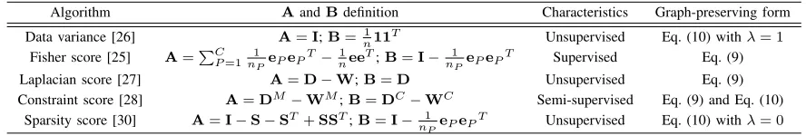
In this section, we will first review some related filter-based feature selection methods. We list some important notions in Table I for ease of explanation. The capital and lower boldface case in this paper denote matrix and vector, respectively.

Data variance [26] is the simplest evaluation criterion for feature selection, reflecting its representative power. We denote

the variance of r-th feature as Varr, which is computed as

follows:

Varr=

1

n n

∑

i=1

(fri−µr)2, (1)

where µr = 1_n

∑n

(3)

TABLE I NOTATIONS

Notation Description

C number of classes

d feature’s dimensionality

xi thei-th sample, wherexi∈Rd

X data matrix, whereX= (x1,x2, . . . ,xn)

fr ther-th feature of all the data

fP

r ther-th feature of theP-th class

fri ther-th feature of thei-th sample

fP

ri ther-th feature of thei-th sample in theP-th class

µr centroid of ther-th feature

µPr centroid of ther-th feature in theP-th class

µ centroid of all samples

n number of samples

nP number of samples in theP-th class

I identity matrix

1 a vector with all elements equal to 1

eP eP(i) = 1if thei-th sample belongs to theP-th class, otherwiseeP(i) = 0 e e= (e1,e2, . . . ,eC)

Fisher score [25] is a supervised feature selection method. It measures the representative power of the feature by assessing its ability of maximizing the distances of the sample from different classes and minimizing the distances of the sample

from the same class simultaneously. LetFSrdenote the Fisher

score of ther-th feature. TheFSr is computed as follow:

FSr=

∑C P=1(µ

P r −µr)2

∑C P=1

∑nP

i=1(friP−µPr)2

, (2)

whereµP

r = n1P

∑nP i=1f

P ri.

Laplacian score [27] is an unsupervised feature selection method. The main idea of Laplacian score is that the data points which locate nearby are probably related to the same class. Therefore, the local structure of the data is more important than the global structure. In this way, Laplacian score evaluates the feature by its ability of preserving the

local structure. The measurement LSr of the r-th feature is

computed as follows:

LSr=

∑n i=1

∑n

j=1(fri−frj)2wij

∑n

i=1(fri−µr)2dii

, (3)

whereD is a diagonal matrix with elementsdii=

∑n j=1wij

andwij is the neighborhood relationship betweenxi andxj.

It is defined as

wij=

      

e−

∥x_i−x_j∥2

t2 if x_i andx_j are neighbors,

0 otherwise,

(4)

where t is a constant set manually. The local structure is

characterized by “if xi and xj are neighbors”. In practice,

δ-ball and K-nearest neighbors are two popular methods

of implementation. We denote the weight matrix W =

(w1,w2, . . . ,wn), then D = Diag(W1), where Diag(·) denotes a diagonal matrix with the elements in the vector.

Constraint score [28] is a supervised feature selection method which can work with partial label information. It employs the pairwise constraints which specify whether a pair of data samples belong to the same class (must-link

constraints) or different classes (cannot-link constraints). The pairwise constraints use much less label information than other supervised methods. Zhang et al. [28] presented two kinds of

constraint scores,CS1_randCS2_r, to measure the importance of

ther-th feature. They are defined as

CS1_r= ∑

(xi,xj)∈M(fri−frj) 2

∑

(xi,xj)∈C(fri−frj)

2, (5)

CS2_r= ∑

(xi,xj)∈M

(fri−frj)2−λ

∑

(xi,xj)∈C

(fri−frj)2, (6)

where M = {(xi,xj)|xi and xj belong to the same class}

is the must-link constraints, C={(xi,xj)|xi andxj belong

to different class} is the cannot-link constraints, and λ is a

parameter to balance the two terms in Eq. (6).

Much attention has been devoted to the sparsity linear representation in these years. It is believed that the sparsity can improve the robustness of the model against data noise. Based on this observation, Liu et al. [30] proposed an unsupervised filter-based feature selection method named as sparsity score.

They first construct al1graph Swith the below method:

min

si

∥si∥1, s.t.xi =Xsi, n

∑

j=1

sij = 1, (7)

where si = (si,1, . . . , si,i−1,0, si,i+1, . . . , si,n)T and S =

(s1,s2, . . . ,sn)T. Then, the measurement SSr of the r-th feature is computed as

SSr1=

∑n i=1

(

fri−

∑n

j=1sijfrj

)2

1 n

∑n

i=1(fri−µr)2

. (8)

In [30], Liu et al. also proposed a filter-based graph-preserving feature selection framework as follows:

score1_r=f

T rAfr fT

rBfr

, (9)

1_{In [30], the authors proposed two SS formulae, namely, SS-1 and SS-2.}

(4)

score2_r=f_rTAfr−λfrTBfr, (10)

whereλis a parameter to balance the two terms in Eq. (10).

Then, the aforementioned feature selection can be unified into

this framework. We list the definitions of Aand B in Table

II. In this table, DM _{= Diag(}_WM₁₎_, _DC _{= Diag(}_WC₁₎

and the elements in matrixWM _and_WC _{are computed as:}

w_ijM =     

1 if (xi,xj)∈Mor (xj,xi)∈M,

0 otherwise,

wCij=

    

1 if (xi,xj)∈C or (xj,xi)∈C,

0 otherwise.

III. THE PROPOSED METHODS

A. Problem formulation

Among various manifold learning algorithms, LLE is one of the most popular methods. LLE first learns the local structure of the data in the original space, then finds their lower-representations by preserving these structures. In the previous work [38], LLE has been embedded into the graph framework for feature extraction. Hence, extending LLE to filter-based feature selection task does not seem to be complicated. How-ever, to our best knowledge, we have not found any work using LLE to rank the feature so far. In this paper, we first introduce how to embed LLE into the graph-preserving framework. To do so, we first model the local structure as what LLE does, which is summarized as below.

For each data point xi,

1) Find the neighborhood set Ni = {xj, j ∈ Ji} using

K-nearest neighbors ofxi.

2) Compute the reconstruction weights that minimize the

reconstructing error ofxi using samples inNi.

Step 1) is usually implemented by employing the Euclidean

distance to find the neighbors. Based on the obtainedKnearest

neighbors, step 2) aims to find the best reconstruction weights. The optimal weights are determined by solving the following problem:

min

{mij, j∈Ji}

∥xi−

∑

j_∈Ji

mijxj∥2, s.t.

∑

j_∈Ji

mij = 1. (11)

Repeating steps 1) and 2) for all the samples, the

reconstruc-tion weights form a weighting matrix M = [mij]n_×n. In

matrix M, mij = 0, if xj ∈ N/ i. It is worth noting that

the dimensionality of the sample d is usually larger than the

numbers of the neighborhoods K, which is d > K. So, the

least squares method is always adopted to solve Eq. (11). Then, each feature is evaluated by its ability to preserving

these weights. We denote Scorer as the measurement of the

r-th feature, which should be minimized, as follows:

Scorer= n

∑

i=1

(

fri− n

∑

j=1 mijfrj

)2

=f_rT(I−M−MT+MTM)fr. (12)

Then we rank the features according to their Scorer, and

choose the top d features with lowest scores. The detailed

procedure of the above method is presented in Algorithm 1.

LetA=I−M−MT₊_MT_M_,_λ_{= 0}_{, the proposed method}

can be embedded into the aforementioned framework in Eq. (10).

Algorithm 1Embedding LLE into the graph-preserving fea-ture selection framework

Input: The data matrixX.

Output: The ranked feature list.

1: Firstly, computeK-nearest neighbors ofxi, then calculate

its reconstruction weightsmij through Eq. (11). Do these

two procedures for all the data, and the weighting matrix

M is obtained;

2: Compute the importance of the dfeature by Eq. (12);

3: Rank the d feature in ascending order according to its

score;

4: return The ranking list of the feature.

Embedding LLE into the graph-preserving feature selection framework is summarized as Algorithm 1. Actually, the score obtained by Algorithm 1 is related to sparsity score. At the first step, both Algorithm 1 and sparsity score construct the reconstruction matrix. Then the features are measured by their abilities of preserving the obtained reconstruction matrix. In

Algorithm 1, each sample is reconstructed by its K-nearest

neighborhoods, which is a local method. Because the number

of nearest neighbor K is always far smaller than the total

number of training samplesn(K≪n), the weighting matrix

M is also sparse. Therefore, compared with sparsity score,

Algorithm 1 provides a very different way to keep the sparsity. Recalling Eq. (7) and Eq. (11), we can find that Algorithm 1 has two advantages over sparsity score. First, the computa-tional cost of Algorithm 1 is much smaller than sparsity score. In sparsity score, each sample is represented by all training samples. It will be time-consuming when the size of training

samples becomes large. Since K is far smaller than the total

number of training samplesn, the computational time of

Algo-rithm 1 will increase slowly, in contrast to sparsity score when the size of training samples gets large. Second, Algorithm 1 is expected to outperform sparsity score in classification tasks. In sparsity score, each sample is represented by all training samples. In this case, a sample is sparsely represented by the training samples, but actually parts of the training samples might be far away from the given sample. In Algorithm 1, the

sample is reconstructed by itsK-nearest neighbors. It has been

proved in [37] that using the K-nearest neighbors to replace

the sparse representation to reconstruct a sample can get better performance in classification tasks. The experimental results in Section 4 also support our analysis.

(5)

TABLE II

THE DEFINITIONS OFAANDBFOR SEVERAL FILTER-BASED FEATURE SELECTION ALGORITHMS

Algorithm AandBdefinition Characteristics Graph-preserving form

Data variance [26] A=I;B= 1

n11

T _Unsupervised _{Eq. (10) with}_λ_{= 1}

Fisher score [25] A=∑C_P₌₁_n1

PePeP

T₋1

nee

T_;_B₌_I₋ 1

nPePeP

T _Supervised _{Eq. (9)}

Laplacian score [27] A=D−W;B=D Unsupervised Eq. (9)

Constraint score [28] A=DM−WM;B=DC−WC Semi-supervised Eq. (9) and Eq. (10)

Sparsity score [30] A=I−S−ST₊_SST_;_B₌_I₋ 1

nPePeP

T _Unsupervised _{Eq. (10) with}_λ_{= 0}

• When the elements in the feature are all equal (take

fr = 1 for example),Scorer = 0 due to the constraint

∑

j∈Jimij = 1, which means the given feature is among

one of the best choice (due toScorer≥0). However, we

know that the feature whose all elements are equal has no discriminant information for classification.

• The measurement Scorer is not scaling invariant. For

example, let f1 = 2×f2, then Score1 = 4×Score2.

Nevertheless, we know that f1 and f2 share the same

graph structures. In other words, f1 andf2 should have

the same ranking score in the feature selection procedure.

• The measurement in Eq. (12) may not capture the change

of the graph efficiently. A toy example is shown in Fig. 1. In the example, the 2-nearest neighbors are employed to model the local structure of the data. We can see that the 2-nearest neighbors of sample 1 are samples 2 and 3 in

R2_{. When we measure the importance of element that lies}

in X1, the 2-nearest neighbors of sample 1 are samples

4 and 5 in the subspace spanned by X1. However, the

measurement in Eq. (12) could not capture this change. Ideally, the preserving ability of the feature should take the change into consideration.

Because of these weaknesses, the score obtained by Algo-rithm 1 may fail in some cases so that its performance will degrade. To solve these problems, we propose a new criterion in next subsection.

B. LLE score

In Section 3.1, the weaknesses of embedding LLE into the graph-preserving framework are already presented. To address these problems, we propose a new criterion to measure the importance of the feature. In the new criterion, we first

compute the reconstruction weights for each element in fr as

follows:

min

{mˆr ij,j∈Jˆi}

∥fri−

∑

j∈Jˆi

ˆ

mr_ijfrj∥2+γ

∑

j∈Jˆi

( ˆmr_ij)2,

s.t. ∑ j∈Jˆi

ˆ

mr_ij = 1,

(13)

where the neighborhood index set Jˆi :={j:if frj is one of

the K-nearest neighbors of fri}. The regularization term in

Eq. (13) is used to make its solution not too sparse, and we will

explain it later in this section. In practice,γis set to be a small

positive value. Using Eq. (13), the reconstruction weighting

matrixMˆr_{= [ ˆ}_mr

ij]for ther-th feature is obtained. Then, we

use the difference betweenMˆrandMto evaluate the

[image:5.612.82.526.83.158.2]

graph-preserving ability of ther-th feature. Here, the Frobenius norm

Fig. 1. A toy example embedding LLE score into the graph-preserving framework could not capture the true change of the structure of the graph.

of the matrix is employed in the proposed method. We denote

LLESr as the score of the r-th feature, which should be

minimized. It is computed as

LLESr=∥M−Mˆr∥2F. (14) For each feature, we use the above criterion to evaluate its ability to preserve the linear structure. The features with small

scores are preferred. We list the details of the proposed LLE

Score in Algorithm 2.

Algorithm 2 LLE score

Input: The data matrixX.

Output: The ranked feature list.

1: Firstly, perform Step 1 of Algorithm 1 to obtain the

weighting matrix M.

2: For eachfr, recompute itsK-nearest neighborhood setNˆi

and reconstruction matrixMˆrvia Eq. (13). Then its LLE

score is calculated for each feature of using Eq. (14);

3: Rank thedfeature in ascending order according to its LLE

score;

4: return The ranking list of the feature.

It is worth noting that when K > 2, problem (13) with

(6)

Lemma 1. Problem (13) with γ = 0 always has multiple solutions whenK >2.

Proof. Problem (13) with γ = 0 takes the form of the following quadratic program

min

y∈RK∥Gy−b∥

2_, _s_._t_.₁T_y_{= 1}_, ₍₁₅₎

where y = [mij]_j_∈_Jˆ_i,G= [frj]_j_∈_Jˆ_i ∈ R1,K,b =fri ∈ R.

Let Z ∈ RK,K−1 _{be the basis matrix of the null space of}

1. With the transformation y =Zyˆ, where yˆ ∈ RK−1 _{is a}

feasible solution of problem (15), we obtain the equivalent form of problem (15) as

min

ˆ

y∈RK−1∥GZˆy−b∥

2_. ₍₁₆₎

Noting thatGZ∈R1,K−1_{and with}_{K >}₂_{, we conclude that}

problem (16) must have multiple solutions, which immediately implies that problem (15) has multiple solutions. The proof is completed.

Consider problem (13) with γ > 0. In this case, the

objective function in problem (13) is strongly convex, and hence Eq. (13) always has a unique solution.

Recalling the aforementioned weaknesses of Algorithm 1, we can see that the improved method overcomes them

effi-ciently. When the elements are all equal, _K1 are assigned to

each neighbor when computing the weights mˆi of the i-th

sample, so that the measurement generally will not be 0. The scaling problem is also solved because we use the weights to measure the feature’s importance, and the computing method for the reconstruction weights are scaling invariant. The last weakness is also solved if we recompute the weights in LLE score. As for the example in Fig. 1, when we evaluate the

importance of element in X1, the neighbors of sample 1 are

recalculated. In this way, the true structure inX1 is captured.

It should be noted that Laplacian score also takes the first two weaknesses into consideration. In their method, the means of the feature are first removed. By doing so, the first problem becomes a trivial solution. The variance of each feature is also used in their method, so the second problem of Algorithm 1 is also solved. We do not use this method in LLE score because the third problem of Algorithm 1 cannot be solved in this way. In general, the proposed scheme in LLE score can solve the three problems of Algorithm 1 simultaneously.

We can also understand the new measurement in LLE score from another perspective. The metric in Eq. (12) calculates

the reconstruction error of fr, which is related to the

graph-structure preserving ability. In the new criterion, we directly evaluate the difference of the two graphs, which is much closer to the aim of the graph-structure preserving ability.

Now, we analyze the time complexity of LLE score. In LLE score, we first compute the reconstruction matrix

M in Eq.(12). The cost of computing the Euclidean

dis-tances between the i-th sample and the other samples is

O(nd), then finding its K-nearest neighbors costs O(nK).

The cost of computing the reconstruction weights is O(K3).

Thus, the total computational complexity of computingM is

O(n2_d₊_n2_K₊_nK3₎_{. To rank each feature, the computational}

complexity for Mˆr is O(n2K+nK3), and for LLESr is

O(n2₎_{. So, to rank each feature, the computational complexity}

is O(n2_K₊_nK3₎_{. The total computational complexity for}

ranking thedfeature isO(n2_d₊_n2_K₊_nK3₊_n2_dK₊_ndK3₎_.

In most cases, d ≫ K, in this way, the computational

complexity can be written into O(n2_d₊_ndK3₎_.

The computational complexity of Algorithm 1 isO(n2d+

ndK3). The computational cost for variation, Laplacian

s-core, and sparsity score are O(n2d), O(n2d), and O(n2d),

respectively. We can see the LLE score is the most time-consuming one among the aforementioned algorithms, where the procedure of computing the reconstruction weights costs most of the extra time.

IV. EXPERIMENTAL RESULTS

In the experiments, we evaluate the performance of LLE score and Algorithm 1 on UCI Iris data set and four image data sets (Yale and ORL face image data sets, COIL20, which is an object image database and MINST, which is a handwriting digit image data set). The properties of them are summarized in Table III. Because we are particularly interested in the learning abilities of unsupervised methods in the classification tasks, only unsupervised methods, such as Variance [26], Laplacian score [27], and sparsity score [30], are included in

the experiments. In the experiments on image data sets, K

-nearest neighbors are used to construct graphs for Laplacian s-core, sparsity ss-core, and our two proposed algorithms. Without

otherwise specified, we setK= 5 in all the algorithms. The

regularization parameterγis set to be10−5_{, which follows the}

conclusion in [39]. The parametert in (4) is searched in the

set{1,10,50,100,200}in Laplacian score, and the best result

is presented. Because we mainly concern the performances of these unsupervised learning methods on classification tasks, the Nearest Class Mean (NCM) classifier and the Nearest Neighbor (NN) classifier are adopted in all the tests for its simplicity. NCM is based on Euclidean distance and could be denoted as

disNCM= min

i ∥x−µi∥ 2_,

(17)

In this way, the sample is assigned to the class which has the

minimum distance disNCM.

NN is also based on Euclidean distance and could be denoted as

disNN= min

i ∥x−xi∥

2_. ₍₁₈₎

The sample is classified to the class that the nearest sample

xi belonging to.

TABLE III PROPERTIES OF DATASETS.

Data sets number of samples number of features number of classes

IRIS 150 4 3

Yale 165 1024 15

ORL 400 1024 40

COIL20 1440 1024 20

(7)

A. Experiments on UCI Iris dataset

The UCI Iris dataset is a collection of 3 types of Iris plants, we denote it to be the class in the following context. For each class, there are 50 samples, in which we use the first 30 samples of each class as the training samples and the other 20 samples of each class as testing samples. Each sample contains 4 features, which are sepal length, sepal width, petal length, and petal width. We use the NCM classifier with each feature, and the classification rates are 0.7333, 0.5833, 0.9667 and 0.9667, respectively. We can see that the discriminative abilities of the 3rd feature and the 4th feature are better than the ones of the 1st feature and the 2nd feature.

We first evaluate the judgement capabilities of the discrim-inative power for each feature of variance, Laplacian score,

sparsity score, Algorithm 1, and LLE score. We setK= 5for

Laplacian score, sparsity score, Algorithm 1, and LLE score.

For Laplacian score, we set t = 10. We list the indexes of

the ranked feature learnt by each algorithm in Table IV. From the results, it is clear that LLE score and sparsity score can evaluate the discriminative power of each feature perfectly. It proves the effectiveness of our proposed scheme in Section 3.2.

We then check the impact ofKon Laplacian score, sparsity

score, Algorithm 1, and LLE score when ranking the features.

We varyKfrom 2 to 20, and list several of them in Table V.

From the results, when K = 2, we find that the features are

ranked as4,3,1,2 by LLE score. This is also a good ranking

according to the classification rates of each feature. In other

situations, the features are all ranked as 3,4,1,2. We can see

that the performance of LLE score is robust to the number of

neighbors K.

B. Experiments on Yale dataset

The Yale face image dataset [40] contains 165 gray scale images from 15 individuals. There are 11 images per person under different face expressions, illumination conditions, and

poses. The images are cropped to32×32pixels with 256 gray

levels per pixel.

In the experiments, we represent the image with its pixel and no further preprocessing is done. In this way, each image is represented by a 1024-dimensional feature vector. The data set is divided into two parts, one used for training the classifier

and the rest for testing. A random subset withp(=2,3,4,5,6,7)

images per individual is taken with labels to form the training set, and the rest of the database is considered to be the testing

set. For each givenp, there are 50 randomly splits. The splits

are downloaded at http://www.cad.zju.edu.cn/home/dengcai/.

For a givenp, we average the results over 50 random splits.

In all the experiments, we record the average classification accuracies over 1024 subsets to see the overall performances of each algorithm, and the best recognition rates and corre-sponding dimensionalities to compare the potential of each algorithm. The results from variance, Laplacian score, sparsity score, Algorithm 1, and LLE score are listed in Table VI. The recognition accuracies versus different subsets are shown in Figs. 2 and 3.

From the results, we can see that Algorithm 1 has compa-rable performance with sparsity score, and LLE score outper-forms other algorithms in most of the cases. It clearly proves that embedding LLE into the graph-preserving framework is a special kind of sparsity score and shows the validity of the proposed measurement in LLE score.

C. Experiments on ORL face image dataset

There are 400 face images in this dataset [41]. The images are from 40 individuals with different illuminations, facial expressions (open or closed eyes, smiling or not smiling), and facial details (glasses or no glasses). The size of each image

is 112×92 with 256 grey levels per pixel.

In the experiments, the images are cropped into 32×32

with no preprocessing conducted. The experimental design here is the same as before. We apply variance, Laplacian score, sparsity score, LLE score, and Algorithm 1 to select the most important features. The recognition is then carried out by using the selected features. We list the classification results for these methods in Table VII and show the classification accuracies versus different dimensionalities in Figs. 4 and 5. As can be seen, LLE score outperforms other algorithms in most of the cases, and Algorithm 1 also outperforms sparsity score in these experiments.

D. Experiments on COIL20 object images dataset

There are 1440 images from 20 objects in this dataset [42].

The size of each image is 128×128, with 256 grey levels per

pixel. The images are resized into 32 ×32 for convenience.

Thus, each image is represented by a 1024-dimensional vector. In the experiments, we randomly select some samples from each object for training and the others for testing. A random

subset withp(=20, 25, 30, 35, 40, 45) images per object are

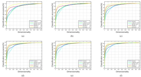
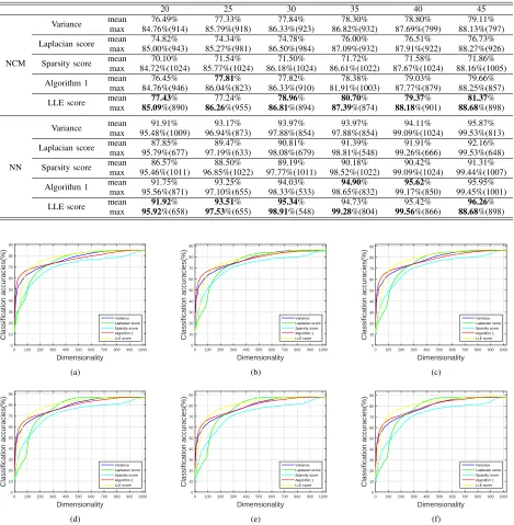
taken as the training set. We repeat this procedure for 25 times. The other experimental designs are the same as before. The experimental results are shown in Table VIII and Figs. 6 and 7. From the results, we can see that LLE score outperforms other algorithms in nearly all the experiments. It proves the effectiveness of the proposed measurement in Eq. (13) and (14).

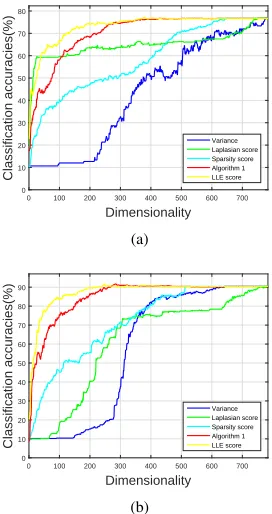
E. Experiments on MNIST handwriting digital image dataset

Finally, we evaluate LLE score on MNIST, which is a well-known handwriting digital image data set. There are 70,000 samples in MNIST, where 60,000 are used for training and the other 10,000 are used for testing. These images are from 10 classes, which are 0-9 digits. The images in this data set

have been size-normalized and centered into 28×28. Thus,

(8)

TABLE IV

THE FEATURE INDEXES OF EACH ALGORITHM ONIRIS DATA SET.

Algorithms Variance Laplacian score Sparsity score Algorithm 1 LLE score Feature indexes 3, 1, 4, 2 2, 1, 4, 3 4, 3, 1, 2 3, 1, 4, 2 3, 4, 1, 2

TABLE V

THE FEATURE INDEXES OF EACH ALGORITHM ONIRIS DATA SET WITH DIFFERENT NUMBER OF NEIGHBORS.

Algorithms Laplacian score Sparsity score Algorithm 1 LLE score

K

2 2, 1, 4, 3 4, 3, 1, 2 3, 1, 4, 2 4, 3, 1, 2

10 4, 3, 1, 2 3, 4, 1, 2 3, 4, 1, 2 3, 4, 1, 2

15 3, 4, 2, 1 4, 3, 1, 2 3, 4, 2, 1 3, 4, 1, 2

20 3, 4, 2, 1 4, 3, 1, 2 3, 1, 4, 2 3, 4, 1, 2

TABLE VI

THE AVERAGE CLASSIFICATION RESULTS ONYALE DATA SET.

2 3 4 5 6 7

NCM

Variance mean 36.02% 41.59% 44.98% 47.11% 49.92% 50.87%

max 43.90%(1022) 52.02%(1024) 56.53%(1023) 58.62%(1016) 62.56%(1020) 63.83%(1022)

Laplacian score mean 39.45% 46.15% 49.94% 53.26% 56.37% 57.82%

max 44.06%(874) 52.25%(1010) 56.61%(974) 59.26%(889) 62.64%(1017) 65.20%(964)

Sparsity score mean 39.30% 46.87% 49.96% 52.63% 54.33% 55.40%

max 42.97%(904) 52.10%(1001) 56.72%(957) 59.04%(927) 62.51%(1023) 63.90%(1018)

Algorithm 1 mean 38.17% 44.29% 48.02% 50.74% 53.78% 55.82%

max 43.91%(1020) 52.07%(1023) 56.51%(1024) 58.64%(1021) 62.56%(1023) 63.86%(1021)

LLE score mean 40.23% 47.36% 51.48% 55.07% 57.90% 60.17%

max 44.37%(849) 52.33%(967) 57.07%(965) 60.15%(799) 62.58%(931) 65.53%(789)

NN

Variance mean 38.72% 44.05% 47.17% 50.30% 52.74% 53.64%

max 45.98%(1004) 51.92%(1019) 54.95%(1020) 58.27%(1010) 61.01%(1010) 62.20%(981)

max 46.58%(846) 52.37%(803) 55.26%(803) 59.22%(806) 61.49%(1017) 62.20%(1005)

max 45.97%(1024) 51.85%(1022) 54.90%(1022) 58.20%(991) 60.80%(1003) 62.20%(1007)

Algorithm 1 mean 42.0303% 47.60% 50.02% 53.88% 56.25% 57.44%

max 45.97%(1023) 52.12%(1002) 55.14%(967) 58.91%(951) 61.17%(947) 62.47%(950)

LLE score mean 43.16% 48.85% 51.40% 54.84% 57.58% 58.17%

max 46.62%(838) 52.58%(824) 55.45%(877) 59.11%(998) 61.93%(853) 62.59%(993)

Dimensionality

0 100 200 300 400 500 600 700 800 900 1000

Classification accuracies(%)

0 5 10 15 20 25 30 35 40 45

Variance Laplasian score Sparsity score Algorithm 1 LLE score

(a)

Dimensionality

0 100 200 300 400 500 600 700 800 900 1000

0 10 20 30 40 50

(b)

Dimensionality

0 100 200 300 400 500 600 700 800 900 1000

0 10 20 30 40 50 60

(c)

Dimensionality

0 100 200 300 400 500 600 700 800 900 1000

0 10 20 30 40 50 60

(d)

Dimensionality

0 100 200 300 400 500 600 700 800 900 1000

0 10 20 30 40 50 60

(e)

Dimensionality

0 100 200 300 400 500 600 700 800 900 1000

0 10 20 30 40 50 60 70

(f)

(9)

Dimensionality

0 100 200 300 400 500 600 700 800 900 1000

0 5 10 15 20 25 30 35 40 45 50

(a)

Dimensionality

0 100 200 300 400 500 600 700 800 900 1000

0 10 20 30 40 50

(b)

Dimensionality

0 100 200 300 400 500 600 700 800 900 1000

0 10 20 30 40 50 60

(c)

Dimensionality

0 100 200 300 400 500 600 700 800 900 1000

0 10 20 30 40 50 60

(d)

Dimensionality

0 100 200 300 400 500 600 700 800 900 1000

0 10 20 30 40 50 60

(e)

Dimensionality

0 100 200 300 400 500 600 700 800 900 1000

0 10 20 30 40 50 60

(f)

Fig. 3. The average classification results whenp=(a) 2, (b) 3, (c) 4, (d) 5, (e) 6, (f) 7 on Yale data set using NN.

TABLE VII

THE CLASSIFICATION RESULTS ONORLDATASET.

2 3 4 5 6 7

NCM

Variance mean 61.52% 66.82% 69.95% 71.83% 73.04% 74.20%

max 70.61%(1024) 76.26%(1017) 79.98%(1023) 81.82%(1018) 83.51%(1024) 85.20%(1024)

max 70.61%(1024) 76.35%(783) 80.35%(728) 81.58%(742) 83.18%(700) 85.20%(1024)

Sparsity score mean_max _70.61%(1024)60.12% _76.28%(1021)65.36% _80.01%(1021)68.68% _81.83%(1015)70.29% _83.51%(1024)71.72% _85.20%(1024)72.94%

Algorithm 1 mean_max _70.6362.19%_%(1017) _76.28%(1014)67.20% _80.02%(1015)70.18% _81.9172.39%_%(1003) _83.62%(975)73.89% _85.20%(1024)73.18%

LLE score mean_max _70.63%(1022)67.03% _76.3772.83_%(997)% _80.04%(990)75.88% _81.82%(1008)77.69% _83.6779.37_%(1007)% _85.20%(1024)80.33%

NN

Variance mean 63.01% 71.79% 76.89% 71.83% 83.66% 86.40%

max 70.45%(1023) 78.88%(1024) 84.52%(1023) 88.09%(1024) 90.29%(1023) 92.57%(866)

max 70.50%(1003) 78.91%(1005) 84.54%(1022) 88.16%(1022) 90.38%(1018) 92.63%(991)

max 70.45%(1017) 78.88%(1024) 84.49%(1024) 88.15%(874) 90.34%(1006) 92.72%(881)

Algorithm 1 mean 64.40% 73.52% 79.58% 72.39% 86.12% 89.00%

max 70.44%(1021) 78.94%(1014) 84.66%(995) 88.28%(997) 90.42%(970) 92.67%(897)

LLE score mean 67.84% 76.78% 82.28% 77.69% 88.20% 90.82%

max 70.69%(1001) 79.19%(917) 84.68%(970) 88.22%(1003) 90.51%(965) 93.03%(927)

TABLE IX

THE CLASSIFICATION RESULTS ONMNISTDATASET.

NCM NN

mean max mean max

Variance 43.01% 76.70%(775) 57.23% 90.40%(642)

Laplacian score 64.96% 77.20%(773) 60.99% 90.80%(783) Sparsity score 58.39% 76.80%(649) 71.96% 90.40%(512) Algorithm 1 70.28% 76.70%(427) 84.81% 91.80%(285) LLE score 73.19% 77.30%(378) 87.38% 92.00%(247)

F. Conlusions on the experimental results

In general, we can draw conclusions from the experiments as follows.

1) Nearly all the best performances of the listed algorithms are not obtained by including all the features, which validates the efficiency and necessity of the dimension reduction procedure.

2) In all the experiments, Algorithm 1 has comparable or better performance than sparsity score. It is consistent with our analysis about the two algorithms in Section 3.1.

(10)

Dimensionality

0 100 200 300 400 500 600 700 800 900 1000

Classification accuracies(%) 0 10 20 30 40 50 60 70 Variance Laplasian score Sparsity score Algorithm 1 LLE score (a) Dimensionality

0 100 200 300 400 500 600 700 800 900 1000

Classification accuracies(%) 0 10 20 30 40 50 60 70 80 Variance Laplasian score Sparsity score Algorithm 1 LLE score (b) Dimensionality

0 100 200 300 400 500 600 700 800 900 1000

Classification accuracies(%) 0 10 20 30 40 50 60 70 80 Variance Laplasian score Sparsity score Algorithm 1 LLE score (c) Dimensionality

0 100 200 300 400 500 600 700 800 900 1000

Classification accuracies(%) 0 10 20 30 40 50 60 70 80 Variance Laplasian score Sparsity score Algorithm 1 LLE score (d) Dimensionality

0 100 200 300 400 500 600 700 800 900 1000

Classification accuracies(%) 0 10 20 30 40 50 60 70 80 Variance Laplasian score Sparsity score Algorithm 1 LLE score (e) Dimensionality

0 100 200 300 400 500 600 700 800 900 1000

[image:10.612.69.535.59.320.2]

Classification accuracies(%) 0 10 20 30 40 50 60 70 80 90 Variance Laplasian score Sparsity score Algorithm 1 LLE score (f)

Fig. 4. The average classification results forp=(a) 2, (b) 3, (c) 4, (d) 5, (e) 6, (f) 7 on ORL data set using NCM.

Dimensionality

0 100 200 300 400 500 600 700 800 900 1000

Classification accuracies(%) 0 10 20 30 40 50 60 70 Variance Laplasian score Sparsity score Algorithm 1 LLE score (a) Dimensionality

0 100 200 300 400 500 600 700 800 900 1000

Classification accuracies(%) 0 10 20 30 40 50 60 70 80 Variance Laplasian score Sparsity score Algorithm 1 LLE score (b) Dimensionality

0 100 200 300 400 500 600 700 800 900 1000

Classification accuracies(%) 0 10 20 30 40 50 60 70 80 Variance Laplasian score Sparsity score Algorithm 1 LLE score (c) Dimensionality

0 100 200 300 400 500 600 700 800 900 1000

Classification accuracies(%) 0 10 20 30 40 50 60 70 80 90 Variance Laplasian score Sparsity score Algorithm 1 LLE score (d) Dimensionality

0 100 200 300 400 500 600 700 800 900 1000

Classification accuracies(%) 0 10 20 30 40 50 60 70 80 90 Variance Laplasian score Sparsity score Algorithm 1 LLE score (e) Dimensionality

0 100 200 300 400 500 600 700 800 900 1000

Classification accuracies(%) 0 10 20 30 40 50 60 70 80 90 Variance Laplasian score Sparsity score Algorithm 1 LLE score (f)

Fig. 5. The average classification results forp=(a) 2, (b) 3, (c) 4, (d) 5, (e) 6, (f) 7 on ORL data set using NN.

V. CONCLUSION

In this paper, we have proposed a new filter-based unsu-pervised feature selection method named LLE score, which is based on LLE and the graph-preserving feature selection framework. The proposed method can solve the problems existed in directly embedding LLE into the graph-preserving feature selection framework. Specifically, the difference

be-tween structures of the graphs constructed by each feature and the original data was used to measure the importance of each feature. Extensive experimental results have demonstrated the validity of the proposed criterion.

[image:10.612.63.536.354.615.2]

(11)

[image:11.612.71.540.82.561.2]

TABLE VIII

THE CLASSIFICATION RESULTS ONCOIL20DATA SET.

20 25 30 35 40 45

NCM

Variance mean_max _84.76%(914)76.49% _85.79%(918)77.33% _86.33%(923)77.84% _86.82%(932)78.30% _87.69%(799)78.80% _88.13%(797)79.11%

max 85.00%(943) 85.27%(981) 86.50%(984) 87.09%(932) 87.91%(922) 88.27%(926)

max 84.72%(1024) 85.77%(1024) 86.18%(1024) 86.61%(1022) 87.67%(1024) 88.16%(1005)

Algorithm 1 mean 76.45% 77.81% 77.82% 78.38% 79.03% 79.66%

max 84.76%(946) 86.04%(823) 86.33%(910) 81.91%(1003) 87.77%(879) 88.25%(857)

LLE score mean 77.43% 77.24% 78.96% 80.70% 79.37% 81.37%

max 85.09%(890) 86.26%(955) 86.81%(894) 87.39%(874) 88.18%(901) 88.68%(898)

NN

Variance mean 91.91% 93.17% 93.97% 93.97% 94.11% 95.87%

max 95.48%(1009) 96.94%(873) 97.88%(854) 97.88%(854) 99.09%(1024) 99.53%(813)

Laplacian score mean_max _95.79%(677)87.85% _97.19%(633)89.47% _98.08%(679)90.81% _98.81%(548)91.39% _99.26%(666)91.91% _99.53%(648)92.16%

Sparsity score mean_max _95.46%(1011)86.57% _96.85%(1022)88.50% _97.77%(1011)89.19% _98.52%(1022)90.18% _99.09%(1024)90.42% _99.44%(1007)91.31%

Algorithm 1 mean_max _95.56%(871)91.75% _97.10%(655)93.25% _98.33%(533)94.03% _98.65%(832)94.90% _99.17%(850)95.62% _99.45%(1001)95.95%

LLE score mean 91.92% 93.51% 95.34% 94.73% 95.42% 96.26%

max 95.92%(658) 97.53%(655) 98.91%(548) 99.28%(804) 99.56%(866) 88.68%(898)

Dimensionality

0 100 200 300 400 500 600 700 800 900 1000

0 10 20 30 40 50 60 70 80 90

(a)

Dimensionality

0 100 200 300 400 500 600 700 800 900 1000

0 10 20 30 40 50 60 70 80 90

(b)

Dimensionality

0 100 200 300 400 500 600 700 800 900 1000

0 10 20 30 40 50 60 70 80 90

(c)

Dimensionality

0 100 200 300 400 500 600 700 800 900 1000

0 10 20 30 40 50 60 70 80 90

(d)

Dimensionality

0 100 200 300 400 500 600 700 800 900 1000

0 10 20 30 40 50 60 70 80 90

(e)

Dimensionality

0 100 200 300 400 500 600 700 800 900 1000

0 10 20 30 40 50 60 70 80 90

(f)

Fig. 6. The average classification results forp=(a) 20, (b) 25, (c) 30, (d) 40, (e) 45, (f) 50 on COIL20 data set using NCM.

the reconstruction weights and the location of the neighbors. The importance of the two terms might not be equal, and we do not know the effects of them yet. Furthermore, evaluating the subset-level score is proved to be an efficient way to select more discriminative features [43]. We will work on these issues and apply the proposed method to other applications [44], [45] in the future.

REFERENCES

[1] J. Lu, K. N. Plataniotis, and A. N. Venetsanopoulos, “Face recognition using LDA-based algorithms,”IEEE Trans. Neural Netw., vol. 14, no. 1, pp. 195–200, 2003.

[2] C. Yao and G. Cheng, “Approximative Bayes optimality linear discrim-inant analysis for Chinese handwriting character recognition,” Neuro-computing, vol. 207, pp. 346–353, 2016.

[3] J. Ye and J. Liu, “Sparse methods for biomedical data,”ACM SIGKDD Explorat. Newslett., vol. 14, no. 1, pp. 4–15, 2012.

[4] X. Lan, A. J. Ma, and P. C. Yuen, “Multi-cue visual tracking using robust feature-level fusion based on joint sparse representation,” inProc. IEEE Conf. Comput. Vis. Pattern Recognit., 2014, pp. 1194–1201.

[5] X. Lan, A. J. Ma, P. C. Yuen, and R. Chellappa, “Joint sparse repre-sentation and robust feature-level fusion for multi-cue visual tracking,” IEEE Trans. Image Process., vol. 24, no. 12, pp. 5826–5841, 2015. [6] X. Lan, S. Zhang, and P. C. Yuen, “Robust joint discriminative feature

learning for visual tracking,” inProc. Int. Joint Conf. Artif. Intell., 2016, pp. 3403–3410.

(12)

Dimensionality

0 100 200 300 400 500 600 700 800 900 1000

0 10 20 30 40 50 60 70 80 90 100

(a)

Dimensionality

0 100 200 300 400 500 600 700 800 900 1000

0 10 20 30 40 50 60 70 80 90 100

(b)

Dimensionality

0 100 200 300 400 500 600 700 800 900 1000

0 10 20 30 40 50 60 70 80 90 100

(c)

Dimensionality

0 100 200 300 400 500 600 700 800 900 1000

0 10 20 30 40 50 60 70 80 90 100

(d)

Dimensionality

0 100 200 300 400 500 600 700 800 900 1000

0 10 20 30 40 50 60 70 80 90 100

(e)

Dimensionality

0 100 200 300 400 500 600 700 800 900 1000

0 10 20 30 40 50 60 70 80 90 100

[image:12.612.71.535.60.319.2]

(f)

Fig. 7. The average classification results forp=(a) 20, (b) 25, (c) 30, (d) 40, (e) 45, (f) 50 on COIL20 data set using NN.

Dimensionality 0 100 200 300 400 500 600 700

0 10 20 30 40 50 60 70 80

(a)

Dimensionality 0 100 200 300 400 500 600 700

0 10 20 30 40 50 60 70 80 90

(b)

Fig. 8. The average classification results with (a) NCM, (b) NN on MNIST data set.

(AAAI), 2017.

[8] D. Zhang, J. Han, L. Jiang, S. Ye, and X. Chang, “Revealing event saliency in unconstrained video collection,”IEEE Trans. Image Process., vol. 26, no. 4, pp. 1746–1758, 2017.

[9] G. Cheng, P. Zhou, and J. Han, “Learning rotation-invariant convolu-tional neural networks for object detection in vhr optical remote sensing images,”IEEE Trans. Geosci. Remote Sens., vol. 54, no. 12, pp. 7405– 7415, 2016.

[10] X. Lu, Y. Yuan, and P. Yan, “Alternatively constrained dictionary learning for image superresolution,”IEEE Trans. Cybern., vol. 44, no. 3, pp. 366–377, 2014.

[11] X. Lu, X. Li, and L. Mou, “Semi-supervised multitask learning for scene recognition,”IEEE Trans. Cybern., vol. 45, no. 9, pp. 1967–1976, 2015. [12] X. Yao, J. Han, D. Zhang, and F. Nie, “Revisiting co-saliency detection: A novel approach based on two-stage multi-view spectral rotation co-clustering,”IEEE Trans. Image Process., vol. 26, no. 7, pp. 3196–3209, 2017.

[13] A. K. Jain, R. P. W. Duin, and J. Mao, “Statistical pattern recognition: A review,”IEEE Trans. Pattern Anal. Mach. Intell., vol. 22, no. 1, pp. 4–37, 2000.

[14] I. Guyon and A. Elisseeff, “An introduction to variable and feature selection,”J. Mach. Learn. Res., vol. 3, no. Mar, pp. 1157–1182, 2003. [15] ——, “An introduction to feature extraction,” in Feature extraction.

Springer, 2006, pp. 1–25.

[16] H. Motoda and H. Liu, “Feature selection, extraction and construction,” Commun. Inst. Inform. Comput. Machinery, vol. 5, pp. 67–72, 2002. [17] C. Ding and H. Peng, “Minimum redundancy feature selection from

microarray gene expression data,”J. Bioinformatics and Computational Biology, vol. 3, no. 02, pp. 185–205, 2005.

[18] A. Sharma, S. Imoto, and S. Miyano, “A top-r feature selection algorithm for microarray gene expression data,”IEEE/ACM Trans. Comput. Biol. Bioinformat., vol. 9, no. 3, pp. 754–764, 2012.

[19] Y. Yang and J. O. Pedersen, “A comparative study on feature selection in text categorization,” inProc. 14th Int’l Conf. Machine Learning, 1997, pp. 412–420.

[20] C. Shang, M. Li, S. Feng, Q. Jiang, and J. Fan, “Feature selection via maximizing global information gain for text classification,” Knowl.-Based Syst., vol. 54, pp. 298–309, 2013.

[21] Z. Li and J. Tang, “Unsupervised feature selection via nonnegative spectral analysis and redundancy control,”IEEE Trans. Image Process., vol. 24, no. 12, pp. 5343–5355, 2015.

[22] Z. Sun, L. Wang, and T. Tan, “Ordinal feature selection for iris and palmprint recognition,”IEEE Trans. Image Process., vol. 23, no. 9, pp. 3922–3934, 2014.

[23] W. Wang, Y. Yan, S. Winkler, and N. Sebe, “Category specific dictionary learning for attribute specific feature selection,” IEEE Trans. Image Process., vol. 25, no. 3, pp. 1465–1478, 2016.

[image:12.612.103.239.365.622.2]

(13)

[25] Q. Gu, Z. Li, and J. Han, “Generalized fisher score for feature selection,” arXiv preprint arXiv:1202.3725, 2012.

[26] C. M. Bishop, Neural networks for pattern recognition. Oxford university press, 1995.

[27] X. He, D. Cai, and P. Niyogi, “Laplacian score for feature selection.” Proc. Advances in Neural Information Processing Systems, vol. Vol. 18, pp. 507–514, 2005.

[28] D. Zhang, S. Chen, and Z.-H. Zhou, “Constraint score: A new filter method for feature selection with pairwise constraints,”Pattern Recog-nit., vol. 41, no. 5, pp. 1440–1451, 2008.

[29] M. A. Hall, “Correlation-based feature selection of discrete and numeric class machine learning,” in Proc. 17th Int’l Conf. Machine Learning, 2000, pp. 359–366.

[30] M. Liu and D. Zhang, “Sparsity score: A novel graph-preserving feature selection method,”Int. J. Pattern Recognit. Artif. Intell., vol. 28, no. 04, p. 1450009, 2014.

[31] M. Yu, L. Liu, and L. Shao, “Structure-preserving binary representations for rgb-d action recognition,”IEEE Trans. Pattern Anal. Mach. Intell., vol. 38, no. 8, pp. 1651–1664, 2016.

[32] M. Yu, L. Shao, X. Zhen, and X. He, “Local feature discriminant projection,” IEEE Trans. Pattern Anal. Mach. Intell., vol. 38, no. 9, pp. 1908–1914, 2016.

[33] S. T. Roweis and L. K. Saul, “Nonlinear dimensionality reduction by locally linear embedding,”Science, vol. 290, no. 5, pp. 2323–2326, 2000. [34] L. Zhang, C. Chen, J. Bu, D. Cai, X. He, and T. S. Huang, “Active learning based on locally linear reconstruction,”IEEE Trans. Pattern Anal. Mach. Intell., vol. 33, no. 10, pp. 2026–2038, 2011.

[35] X. Liu, D. Tosun, M. W. Weiner, N. Schuff, A. D. N. Initiativeet al., “Locally linear embedding (LLE) for MRI based Alzheimer’s disease classification,”NeuroImage, vol. 83, pp. 148–157, 2013.

[36] J. Ma, H. Zhou, J. Zhao, Y. Gao, J. Jiang, and J. Tian, “Robust feature matching for remote sensing image registration via locally linear transforming,”IEEE Trans. Trans. Geosci. Remote Sens., vol. 53, no. 12, pp. 6469–6481, 2015.

[37] N. Zhang and J. Yang, “K nearest neighbor based local sparse represen-tation classifier,” inIEEE Chine. Conf. on Pattern Recognition CCPR. IEEE, 2010, pp. 1–5.

[38] J. B. Tenenbaum, V. De Silva, and J. C. Langford, “A global geometric framework for nonlinear dimensionality reduction,”Science, vol. 290, no. 5, pp. 2319–2323, 2000.

[39] G. H. Golub, P. C. Hansen, and D. P. O’Leary, “Tikhonov regularization and total least squares,”SIAM J. Matrix Anal. App., vol. 21, no. 1, pp. 185–194, 1999.

[40] P. N. Belhumeur, J. P. Hespanha, and D. J. Kriegman, “Eigenfaces vs. fisherfaces: Recognition using class specific linear projection,” IEEE Trans. Pattern Anal. Mach. Intell., vol. 19, no. 7, pp. 711–720, 1997. [41] F. S. Samaria and A. C. Harter, “Parameterisation of a stochastic model

for human face identification,” inProc. IEEE Workshop Applications of Computer Vision. IEEE, 1994, pp. 138–142.

[42] S. A. Nene, S. K. Nayar, H. Murase et al., “Columbia object image library (coil-20),” Technical Report CUCS-005-96, Tech. Rep., 1996. [43] F. Nie, S. Xiang, Y. Jia, C. Zhang, and S. Yan, “Trace ratio criterion for

feature selection.” inProc. Conf. Artificial Intelligence (AAAI), vol. 2, 2008, pp. 671–676.

[44] D. Zhang, J. Han, C. Li, J. Wang, and X. Li, “Detection of co-salient objects by looking deep and wide,”Int. J. Comput. Vis., vol. 120, no. 2, pp. 215–232, 2016.

[45] D. Zhang, J. Han, J. Han, and L. Shao, “Cosaliency detection based on intrasaliency prior transfer and deep intersaliency mining,”IEEE Trans. Neural Netw. Learn. Syst., vol. 27, no. 6, pp. 1163–1176, 2016.

Chao Yaoreceived his B.Sc. in telecommunication engineering in 2007, and the Ph.D. degree in com-munication and information systems in 2014, both from Xidian University, Xi’an, China. He was a visiting student in Center for Pattern Recognition and Machine Intelligence (CENPARMI), Montreal, Canada, during 2010-2011. Now he is a Postdoctoral Fellow at Northwestern Polytechnical University, Xi’an, China. His research interests include feature extraction, handwritten character recognition, ma-chine learning, and pattern recognition.

Ya-Feng Liu(M’12) received the B.Sc. degree in applied mathematics in 2007 from Xidian University, Xi’an, China, and the Ph.D. degree in computational mathematics in 2012 from the Chinese Academy of Sciences (CAS), Beijing, China. During his Ph.D. study, he was supported by the Academy of Mathe-matics and Systems Science (AMSS), CAS, to visit Professor Zhi-Quan (Tom) Luo at the University of Minnesota (Twins Cities) from February 2011 to February 2012. After his graduation, he joined the Institute of Computational Mathematics and Scien-tific/Engineering Computing, AMSS, CAS, Beijing, China, in July 2012, where he is currently an Assistant Professor. His main research interests are nonlinear optimization and its applications to signal processing, wireless communications, machine learning, and image processing. He is especially interested in designing efficient algorithms for optimization problems arising from the above applications.

Dr. Liu is currently serving as the guest editor of the Journal of Global Optimization. He is a recipient of the Best Paper Award from the IEEE International Conference on Communications (ICC) in 2011 and the Best Student Paper Award from the International Symposium on Modeling and Optimization in Mobile, Ad Hoc and Wireless Networks (WiOpt) in 2015.

Bo Jiangreceived the B.Sc. degree in applied math-ematics in 2008 from China University of Petroleum, Dongying, China and the Ph.D. degree in com-putational mathematics in 2013 (advisor Prof. Yu-Hong Dai) from the Chinese Academy of Sciences (CAS), Beijing, China. After graduation, he was a postdoc with Professor Zhi-Quan (Tom) Luo at the University of Minnesota (Twins Cities) from September 2013 to March 2014. He has been a lecturer at School of Mathematical

Jungong Hanis a faculty member with the School of Computing and Communications at Lancaster University, Lancaster, UK. Previously, he was a faculty member with the Department of Computer and Information Sciences at Northumbria University, UK.