Manuscript version: Author’s Accepted Manuscript
The version presented in WRAP is the author’s accepted manuscript and may differ from the published version or Version of Record.
Persistent WRAP URL:
http://wrap.warwick.ac.uk/128480
How to cite:
Please refer to published version for the most recent bibliographic citation information. If a published version is known of, the repository item page linked to above, will contain details on accessing it.
Copyright and reuse:
The Warwick Research Archive Portal (WRAP) makes this work by researchers of the University of Warwick available open access under the following conditions.
Copyright © and all moral rights to the version of the paper presented here belong to the individual author(s) and/or other copyright owners. To the extent reasonable and
practicable the material made available in WRAP has been checked for eligibility before being made available.
Copies of full items can be used for personal research or study, educational, or not-for-profit purposes without prior permission or charge. Provided that the authors, title and full
bibliographic details are credited, a hyperlink and/or URL is given for the original metadata page and the content is not changed in any way.
Publisher’s statement:
Please refer to the repository item page, publisher’s statement section, for further information.
Electric field stabilization of viscous liquid layers coating the
underside of a surface
Thomas G. Anderson
Department of Computing & Mathematical Sciences,
California Institute of Technology, Pasadena, CA 91125, United States
Radu Cimpeanu and Demetrios T. Papageorgiou
Department of Mathematics, Imperial College London,
SW7 2AZ, London, United Kingdom
Peter G. Petropoulos
Department of Mathematical Sciences,
New Jersey Institute of Technology, Newark, NJ 07102, United States
(Dated: November 15, 2016)
Abstract
We investigate the electrostatic stabilization of a viscous thin film wetting the underside of a
hori-zontal surface in the presence of an electric field applied parallel to the surface. The model includes
the effect of bounding solid dielectric regions above and below the liquid-air system that are typically
found in experiments. The competition between gravitational forces, surface tension and the non-local
effect of the applied electric field is captured analytically in the form of a nonlinear evolution equation.
A semi-spectral solution strategy is employed to resolve the dynamics of the resulting partial
differ-ential equation. Furthermore, we conduct direct numerical simulations (DNS) of the Navier-Stokes
equations using the volume-of-fluid methodology and assess the accuracy of the obtained solutions in
the long-wave (thin film) regime when varying the electric field strength from zero up to the point
when complete stabilization occurs. We employ DNS to examine the limitations of the asymptotically
derived behavior as the liquid layer thickness increases, and find excellent agreement even beyond
the regime of strict applicability of the asymptotic solution. Finally, the asymptotic and
computa-tional approaches are utilized to identify robust and efficient active control mechanisms allowing the
I. INTRODUCTION
Rayleigh-Taylor instabilities of liquid layers have been studied by numerous authors both theoretically and experimentally. Linear stability analysis and two-dimensional nonlinear com-putations can be found in [1–3], for example, where it is found that dripping transitions take place for sufficiently thick layers with fingers of heavy fluid penetrating lighter fluid. In the case of films thinner than the capillary length (σ/ρg)1/2 (here σ is the surface tension coeffi-cient, ρ is the density and g the gravitational acceleration), dripping does not take place, but instead drops are formed that are connected by slowly draining thinning regions. The thin film models describing such phenomena were derived and studied by Yiantsios & Higgins [1], and interestingly the equations are identical to the axisymmetric capillary film draining equations first studied by Hammond [4] that are driven by capillary instabilities in the absence of gravity. The dynamics of drop formation become much more intricate on longer domains that can allow drops to move within the domain, as shown by accurate computations and analysis by Lister et al. [5]. Motivated by the experiments and weakly nonlinear analyses of Limat and co-workers [6, 7], the one-dimensional patterns studied in [5] were extended to two-dimensional ones by Lister et al. [8] who found new behavior such as droplet coalescence or bouncing.
The stabilization of the gravity-driven Rayleigh-Taylor instability has also been considered by several authors. Babchin et al. [9] showed that a nonlinear saturation is possible in the presence of a constant background shear - this is analyzed for a two-fluid Couette flow with a thin lighter film beneath a heavier upper fluid. Stabilization was also demonstrated by Halpern & Frenkel [10] for cases when the shear arises due to zero-mean time-periodic oscillations of the upper plate of a two-fluid Couette flow. Stabilization has also been predicted theoretically in [11] for liquid films coating the outside surface of a horizontal cylinder performing time-periodic oscillations along its axis.
self-similar forms and their confirmation via numerical computations) were explored in detail in [17], both in the presence and absence of surface tension. If surface tension is present the local geometry of the touching interface maintains bounded gradients but unbounded curva-ture (a corner singularity) with electric field effects being of higher order; for electrified flows with zero surface tension the touching singularities are worse in the sense that cusps form with interfacial gradients blowing up locally. One of the objectives of the present study is to include viscosity and also more realistic electric field configurations. We also note that direct numerical simulations for electrified Rayleigh-Taylor flows that are unbounded in the vertical direction were carried out by Cimpeanu et al. [18] who find complete stabilization of finite wavelength perturbations and in addition quantify the effect of the field on the formation and dynamics of finger formation and propagation of the heavier fluid into the lighter one.
The structure of the paper is as follows. Section II describes the mathematical model and carries out an asymptotic analysis to derive an evolution equation for the dynamics of thin films. Section III presents computations based on the model equation and describes the effect of the electric field on the solutions. Section IV presents direct numerical computations of the problem valid for arbitrary thickness fluid layers and arbitrary Reynolds numbers. A direct comparison between the asymptotic and numerical solutions is also presented. Section V uses the results to suggest an application of utilizing electric fields to produce controlled interfacial oscillations that do not rupture the layer and do not produce dripping. We conclude with a discussion in Section VI.
II. MATHEMATICAL MODEL
II.1. Governing equations
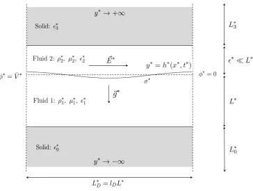
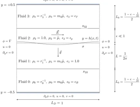
We consider two superposed immiscible fluid layers placed in the gap between two solid dielectric slabs of infinite vertical extent - see the schematic in Fig. 1; the flow is assumed to be two-dimensional. A horizontal electric field driven by lateral electrodes far away is assumed to be present both in the fluids as well as the solid dielectric bounding slabs as shown in the schematic. The dynamics are driven by the competition between gravitational, surface tension and electric field effects, with the latter two acting to stabilize Rayleigh-Taylor instability in an initially quiescent flow.
The overhanging layer (region 2) wetting the underside of the upper slab is a dielectric Newtonian liquid with constant density ρ∗2, viscosity µ∗2 and permittivity ∗2 and lies in h∗ ≤
FIG. 1. Schematic of the problem with fluid 2 lying above fluid 1 and separated by the interface
y∗=h∗(x∗, t∗). A uniform electric field of size E∗ = ¯V∗/L∗D is applied horizontally as shown.
flat lower boundary of the upper solid slab region 3, y∗ > h∗u. The lower dielectric fluid region 1 in 0 ≤ y∗ ≤ h∗ is much less dense and viscous and is hydrodynamically passive to leading order (the negligible physical properties simplify the governing equations to describe a region of zero velocities and uniform pressure); its electrical permittivity is ∗1. This is bounded below by another solid slab denoted by region 0 and lying in y∗ <0. The dielectric permittivities in regions 0 and 3 are ∗0 and ∗3, respectively. In addition surface tension is present with constant coefficient σ∗, and gravity is acting in the vertical direction with constant acceleration g∗. The velocity field in the upper liquid layer is u∗2 = (u∗2, v∗2) and the pressures in regions 1 and 2 are
p∗1,2. The electrodes are kept at constant voltage potentials φ∗ = ¯V∗ on the left and φ∗ = 0 on the right as shown in Fig. 1, resulting in a uniform horizontal electric field of magnitude
E∗ = ¯V∗/L∗D in the undisturbed configuration.
The Navier-Stokes and continuity equations hold in region 2
ρ∗2(u∗2t+ (u∗2· ∇)u∗2) =−∇p∗2+µ∗2∆u∗2−ρ∗2g∗j, (1)
∇ ·u∗2 = 0, (2)
and voltage potentials φ∗0,1,2,3 are present in each region producing an electric field E∗i =−∇φ∗i
each region (this follows from the electrostatic limit of Maxwell’s equations)
∇2φ∗
0,1,2,3 = 0, (3) where ∇2 =∂2
x∗ +∂y2∗. At the interface y∗ = h∗(x∗, t∗) we must impose the balance of normal and tangential stresses,
[n·T∗·n]12 =σ∗κ, [t·T∗·n]12 = 0, (4)
where [(·)]1
2 = (·)1−(·)2 denotes the jump across the interface,n = (−h∗x∗,1)/(1 +h∗x2∗)1/2,t= (1, h∗x∗)/(1 +hx∗2∗)1/2are the unit normal and tangent to the interface, andκ=h∗x∗x∗/(1 +h∗x2∗)3/2 is the interfacial curvature. The stress tensor T∗ contains electric and fluid parts and is given
by
Tij∗ =−p∗δij+ ˜µ∗
∂u∗i ∂x∗j +
∂u∗j ∂x∗i
+∗E˜i∗E˜j∗−1
2 ∗|
E∗|2δij, (5)
where it is understood that the appropriate subscript is used in different regions. As a result of the fluids being perfect dielectrics with constant permittivities, there are no charges present in the flow, and hence the Lorentz force has no contribution in the momentum conservation equation (1). Instead, the jump in Maxwell stresses manifests itself nonlinearly in the stress balance conditions (4). In addition we have a kinematic condition
v∗2 =h∗t∗+u∗2hx∗∗ at y∗ =h∗(x∗, t∗) (6)
and no-slip conditions at the solid wall,
u∗2 =v2∗ = 0 at y∗ =h∗u. (7)
The interfacial boundary conditions for the electric field are Gauss’s law and continuity of the tangential component,
[∗E∗·n]ii+1 = 0, [t·E∗]ii+1 = 0, i= 0, 1, 2. (8)
The second condition is equivalent to
[φ∗]10 = 0, [φ∗]21 = 0, [φ∗]32 = 0. (9)
We non-dimensionalize velocities using the scale U∗ = √g∗L∗ so as to retain the gravity-driven Rayleigh-Taylor instability. The lower fluid layer heightL∗ is used as a reference length-scale, time is scaled by L∗/√g∗L∗, and pressure is scaled according to p∗ ∼ ρ∗
2U∗2 ∼ ρ∗2g∗L∗. The voltage potentials are non-dimensionalized usingV0∗. (In what follows we use the same sym-bols for dimensionless variables but they are un-starred.) The following dimensionless groups emerge from the manipulation of the equations and boundary conditions
˜
g = g ∗L∗
U∗2 ≡1, µ˜=
µ∗2
ρ∗2L∗(g∗L∗)1/2, We =
σ∗
ρ∗2g∗L∗2, Eb =
∗1V∗2 0
These represent the unit inverse square Froude number ˜g, an inverse Reynolds number ˜µ, an inverse Weber number We and an electric dimensionless group Eb. Note that we have used
quantities in the upper fluid layer 2 as reference for hydrodynamic values, while the permittivity
∗1of region 1 is selected as reference, leading to the following relevant relative permittivity ratios
B =∗0/ ∗
1, p =∗2/ ∗
1, T =∗3/ ∗
1. (11)
Hence, the dimensionless Navier-Stokes equations in region 2 become
ut+ (u· ∇)u=−∇p2+ ˜µ∆u−˜gj, (12)
∇ ·u= 0, (13)
where we have removed the subscript 2 since the bottom layer region 1 is hydrodynamically passive. The normal and tangential stress balances at y=h(x, t) (recall eq. (4)) reduce to
−(1 +h2x)(p1−p2) + 2˜µhx(vx+uy)−2˜µ(vy+hx2ux)−2hxEb
∂φ1
∂x ∂φ1
∂y + (14)
+2pEbhx
∂φ2
∂x ∂φ2
∂y +
1 2Eb(h
2
x−1)
∂φ1 ∂x 2 − ∂φ1 ∂y 2 − −1
2pEb(h 2
x−1)
∂φ2 ∂x 2 − ∂φ2 ∂y 2
=We
hxx
(1 +h2
x)1/2
,
2hx(ux−vy)−(1−h2x)(uy+vx) = 0. (15)
Finally, the kinematic condition reads
v =ht+uhx at y=h(x, t). (16)
The Laplace equations (3) for the voltages are unchanged and so are the voltage continuity conditions (9). The latter are simple at the fixed solid boundaries y = 0 and y =hu, while at
the deforming interface voltage continuity takes the form
∂φ2
∂x +hx ∂φ2
∂y = ∂φ1
∂x +hx ∂φ1
∂y at y=h(x, t). (17)
Finally, the Gauss law conditions (continuity of the electric displacement field) become
B
∂φ0
∂y = ∂φ1
∂y at y= 0, (18)
−hxp
∂φ2
∂x +p ∂φ2
∂y =−hx ∂φ1
∂x + ∂φ1
∂y at y=h(x, t), (19)
p
∂φ2
∂y =T ∂φ3
∂y at y=hu. (20)
Using bars to denote the undisturbed state characterized by a flat interface, the above system admits the following exact solution
¯
This solution is unstable and in what follows we present a nonlinear theory valid for thin fluid layers and describe the spatiotemporal dynamics under the action of electric fields. Direct numerical simulations are considered later - see Section IV.
II.2. Evolution equation for thin liquid films
Assume that the upper liquid layer region 2 has mean thickness 1, so that in its undisturbed state it is bounded between y= ¯h = 1 andy=hu = 1 +. We consider interfacial
deflections that have order one wavelengths and order amplitudes, i.e. fully nonlinear in the sense that they scale with the fluid layer thickness. We write the interfacial position as
y=h(x, t) = 1 +˜h(x, t), ˜h(x, t) =O(1). (22)
It is useful to introduce a stretched inner coordinate η given by y = 1 + − η, so that
∂y → −−1∂η. The orderdeflection produces equivalent perturbations to the voltage potentials
and the pressure jump contribution due to surface tension. The appropriate expansions are, therefore,
p1 = ¯p1, p2 = ¯p2+ 1−y+p˜+. . . , φj =x+φ˜
(0)
j +
2φ˜(1)
j +. . . , (23)
where j = 0,1,2,3, and ¯p1, ¯p2 are constants - in fact ¯p2 −p¯1 = Eb(1−p)/2 as follows from
(14) for the base state solution. Note also that the term 1−y in the expression for p2 is the hydrostatic contribution. The Navier-Stokes equations are used next to obtain the scalings for the velocities required for the viscous terms to balance pressure. Under the assumption that the Reynolds number Re = ˜µ−1 =O(1), we find
u=3u˜0+4u˜1+. . . , v =4v˜0+5˜v1+. . . , (24)
with the scaling for v being a direct consequence of mass conservation. Finally, the relevant timescale for the dynamics is found from the kinematic condition, which to leading order reads
3˜v0 = ˜ht+3u˜0˜hx at η= 1−h,˜ (25)
which leads to a slow time scale
τ =3µ˜−1t. (26)
After solving foru0 andv0 from the leading order contributions of the Navier-Stokes equations, and substituting into (25), the following evolution equation for the interface is found
˜
hτ +
∂ ∂x
" ˜
px
(1−˜h)3 3
#
It remains to determine ˜px at the interface in terms of ˜h to obtain a closed system. This is
achieved by expanding the normal stress balance condition (14) to obtain, at leading order,
˜
p= ˜h+We˜hxx+Eb
˜
φ(0)1x
y=1− p ˜
φ(0)2x
η=1−˜h
. (28)
Note that in this expression we have used the solution (35) derived below which ensures that the Maxwell stress contribution φ22y to (14) is of order 2 at most and does not contribute to (28). The horizontal electric field terms ˜φ(0)1x and ˜φ(0)2x need to be determined by solving the system (3) and (20) and their appropriate boundary conditions. The voltage potential in region 1 can be readily solved in Fourier space:
d2φd˜(0) 1
dy2 −k 2φd˜(0)
1 = 0 ⇒ dφ (0)
1 =α(k) cosh(ky) +β(k) sinh(ky), (29)
with α(k) and β(k) to be found (hats denote Fourier transforms in the usual way). The potentials ˜φ1 and ˜φ2 are linked through (19), which on use of the expansions (22) and (23) becomes
−pφ˜
(0) 2η
η=1−˜h− p
˜
hx+ ˜φ
(1) 2η
η=1−˜h
+O(2) =−˜hx−φ˜
(0) 1y y=1
+O(2). (30)
In the thin film region 2, the Laplace equation becomes 2φ
2xx +φ2ηη = 0, and from the
expansions (23) we have
˜
φ(0)2ηη = 0, φ˜(1)2ηη = 0, (31) whose solutions are
˜
φ(0)2 =A0(x, τ)η+B0(x, t), φ˜ (1)
2 =A1(x, τ)η+B1(x, t), (32)
with A0, A1, B0, B1 to be found. An additional coupling to the fields in the slab regions 0 and 3 is present due to the voltage continuity conditions at y= 0,1 +, and the Gauss laws (18) and (20). Following [19] we use the fact that the complex functions ∂xφj −i∂yφj with j = 0,3
are analytic in their respective domains, and apply Cauchy’s theorem in region 0 and 3 in turn. Imposing the voltage continuity conditions at the walls leads to the following non-local boundary conditions, written in unscaled form for the moment,
−B
π P V
+∞ Z
−∞
φ1x(x0,0)
x0−x dx 0
= ∂φ1
∂y y=0
, T
π P V
+∞ Z
−∞
φ2x(x0,1 +)
x0 −x dx 0
=p
∂φ2 ∂y y=1+ , (33)
where PV denotes the principal value of the integral. Introducing the expansions (23) and the inner variable η into (33)b, we find at order 1 and order , respectively,
−pφ˜
(0) 2η
η=0 = 0,
T
π P V Z ∞
−∞
φ(0)2x(x0, η= 0)
x0−x dx 0
=−pφ˜
(1) 2η
The first condition implies that A0(x, τ) = 0 in (32) so that
˜
φ(0)2 =B0(x, τ), (35)
while the second condition yields
T
πP V Z ∞
−∞
B0x(x0, τ)
x0−x dx 0 =−
pA1(x, τ). (36)
Using solutions (32) and (35) into the Gauss law (30) gives
˜
φ(0)1y
y=1 = (1−p)˜hx−pA1, (37) and substituting (29) and (36) and going into Fourier space we find
kα(k) sinh(k) +kβ(k) cosh(k) = ik(1−p)b˜h−T|k|Bc0. (38)
Two more conditions connecting the unknownsα(k),β(k) andBc0(k) arise from the order con-tributions of condition (33)a and continuity of voltage potentials across the fluid-air interface. These are
B|k|dφ
(0) 1 =
dφd(0) 1 dy y=0
, φd(0) 1 y=0
=Bc0. (39)
Solving (38) and (39) allows us to express B0 in terms of ˜h:
b
B(k) = i(1−p)
kcosh(k) +B|k|sinh(k)
(B+T)|k|cosh(k) + (1 +BT)ksinh(k)
b ˜
h. (40)
It also follows from the solutions just obtained that (28) takes the form ˜p= ˜h+We˜hxx+Eb(1−
p)B0x and hence the evolution equation (27) becomes
ht+
1 3
(1−h)3 hx+Wehxxx +Eb(1−p)Bxx
x = 0, (41)
where for simplicity we have dropped the tilde decoration and τ has been replaced by t. The interface will touch the wall if h →1 from below. We describe our numerical solution of (41) in Appendix A. Note that in the absence of the lower dielectric slab (region 0), the non-local expression (40) simplifies to a form that shares strong similarities with the corresponding term in the evolution equation previously derived by Tseluiko & Papageorgiou [20]. In the respective case the sign is shifted due to their destabilizing vertical electric field configuration, while the prefactor is also different, as here we include the influence of the upper solid region 3 through
T. The same result can be retrieved by considering the small wavelength (largek) limit of the
III. NUMERICAL RESULTS FOR THE THIN-FILM EQUATION
In order to gain a fundamental understanding of the competition of the modeled physical phenomena and provide a quantitative basis for subsequent nonlinear computations, we first conduct a linear study of the long-wave evolution equation (41), focusing on the effects of varying the electric field strength. Linearizing about h≡0 and seeking solutions proportional to exp(ωt+ikx), yields the following dispersion relation
ω(k) = 1 3k
2− 1 3Wek
4− 1
3(1−p) 2E
bk3
kcosh(k) +B|k|sinh(k)
ksinh(k)(1 +BT) +|k|cosh(k)(B+T)
. (42)
The first term on the right-hand-side is destabilizing and originates from the gravitational acceleration; the second term accounts for the stabilizing effect of surface tension, while the final term corresponds to the electric field. The five parameters in the system, We, Eb, p, B
and T, are selected as far as possible to correspond to realistic values that could be found in
desktop experiments. Note that in many practical contexts we find that the bounding solid regions are fabricated from the same material, implyingB =T, and thus reducing the number
of parameters even further.
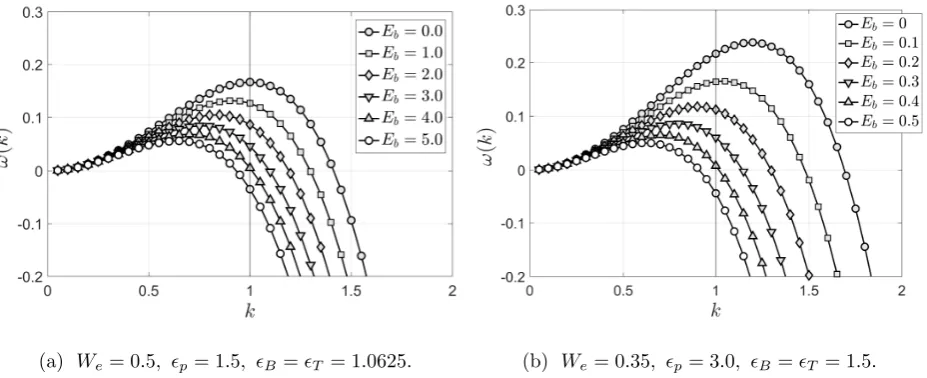
(a) We= 0.5, p = 1.5, B =T = 1.0625. (b) We= 0.35, p= 3.0, B =T = 1.5.
FIG. 2. Linear growth rates, as defined in equation (42), for two example cases, illustrating the
stabilizing effect of the electric field with adjustable strength via the Eb parameter.
We consider two typical but distinct example cases: a) We = 0.5, Eb varying from 0 to
5.0, p = 1.5 and B = T = 1.0625; and, b) We = 0.35, Eb varying from 0 to 0.5, p = 3.0
and B = T = 1.5. The resulting growth rates R(ω(k)) are illustrated in Fig. 2(a)-2(b). The
anticipated behavior of long wave instability over a finite number of unstable modes is observed, with long waves (small k) remaining unstable irrespective of the parameter values and short waves (large k) eventually stabilized by surface tension. Increasing Eb has a stabilizing effect
[image:11.595.68.532.392.581.2]value of Eb was selected so that all waves with k ≥ 1 are linearly stable. In the nonlinear
calculations that follow we fix matters by taking a periodic domain of length 2π so that the mode k = 1 is stable or slightly unstable, depending on the value of Eb. This in turn enables
[image:12.595.67.532.168.374.2]us to use extensive nonlinear calculations to probe the interaction of near-wall dynamics with the electric field.
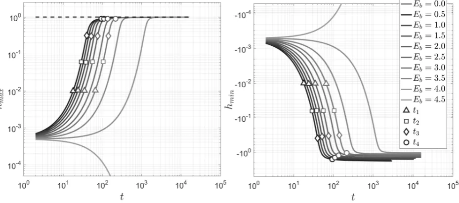
FIG. 3. Evolution of maximum hmax(t) and minimum hmin(t) positions of the interface in time for
We = 0.5, p = 1.5, B =T = 1.0625 and varying Eb.
For case a) above, an electric field strength of Eb = 4.5 is found to be sufficient to completely
suppress the instability. Hence we carry out a number of calculations of (41) for 0≤Eb ≤4.5
in order to study features beyond the linear regime. The domain is fixed to be 2π−periodic and the initial condition used is
h(x,0) = −5·10−4 cosx, (43)
so that its minimum is in the center of the computational domain and its amplitude is small enough to allow the instability to grow through its linear stage when unstable.
Fig. 3 presents the dynamics of the interface as a function of time and electric field strength. The left panel depicts the interfacial maximum denoted by hmax and the right panel the
inter-facial minimum hmin. In the cases where Eb <4.5, an initial linear exponential growth occurs
until the interface encounters the upper wall and then converges slowly to a state wherehmax(t) is asymptotically close toy = 1; at the same time,hmin(t) reaches a value which depends onEb.
wall. For example, the number of dimensionless time units required for the interfacial maximum
hmax to reach y = 0.9 is 94 when Eb = 0.0, and increases to 2000 when Eb = 4.0 which is the
final computation considered before Eb becomes sufficiently high so as to stabilize the interface
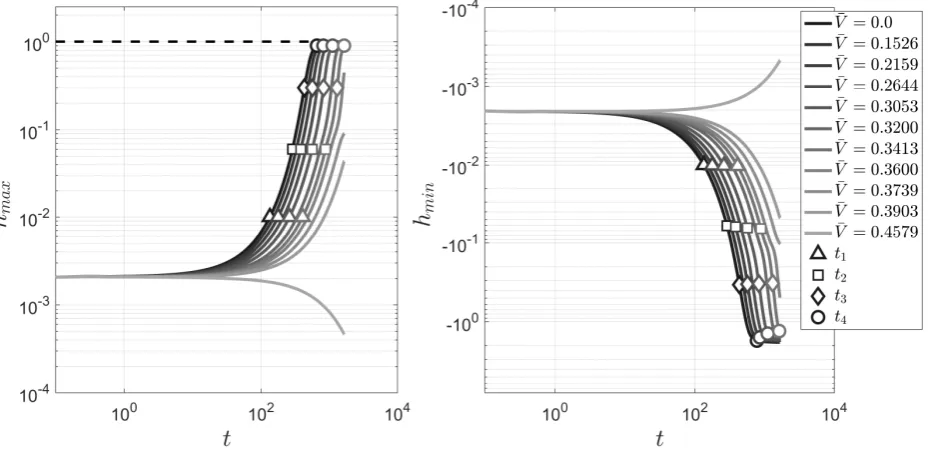
to a flat state. Several points in the figure have been marked with symbols to serve as points of comparison with subsequent direct numerical simulations. We define ti to denote the first
time at which hmax exceeds a given threshold yi, with four such values chosen as y1 = 10−2,
y2 = 6·10−2, y3 = 5·10−1 and y4 = 9·10−1; the last value is sufficiently close to the wall such that nonlinear features become prominent. We emphasize that the nonlinear draining be-haviour described in this confined system is in qualitative contrast with the evolution into the well-known ”mushroom” shape of the Rayleigh-Taylor instability found in vertically unbounded domains [18]. In the present study the liquid films are not thick enough to support dripping dynamics; instead the fluid gathers into structures comprising of collars and smaller amplitude secondary lobes separated by slowly thinning regions [5].
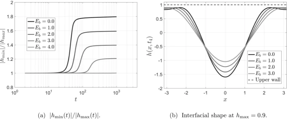
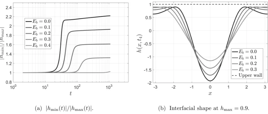
[image:13.595.65.526.343.538.2](a) |hmin(t)|/|hmax(t)|. (b) Interfacial shape athmax= 0.9.
FIG. 4. Shape dynamics for We = 0.5, p = 1.5, B =T = 1.0625.
Our computations indicate that one of the main properties affected by the electric field is the geometry of the evolving interface as measured by aspect ratio χ =|hmin(t)|/|hmax(t)|, for example; this serves as a measure of the distortion of the interface when compared to its initial regular cosine profile. Results corresponding to case a) parameters are given in Fig. 4(a). In the absence of electric effects, Eb = 0, the nonlinear stage starts at t ≈ 20.0 and we find a
secondary lobe containing a (relatively) small amount of fluid. The electric field acts towards a delay in the onset of the formation of this structure, which also leads to a reduction in size of the volume of fluid within. Comparing interfacial shapes with the same hmax during their
evolution, we find that asEb increases the two maxima are found closer to±π, and forEb = 4.0
the initial cosine shape is actually retained until the end of the computation. Referring back to Fig. 4(a), |hmin(t)|/|hmax(t)| decreases steadily as a function of Eb down to unity, which
indicates regularization to a sinusoidal shape of the interface as the electric field contribution is increased.
[image:14.595.66.526.235.431.2](a) |hmin(t)|/|hmax(t)|. (b) Interfacial shape athmax= 0.9.
FIG. 5. Shape dynamics forWe= 0.35, p = 3.0, B=T = 1.5.
A similar trend is found for the second choice of parameters, case b) above, with the inter-facial extrema dynamics shown in Fig. 5(a)-Fig. 5(b). In this case the surface tension effects are smaller and the nonlinearity in the interface becomes more pronounced, with χ reaching 2.2 when no electric field is present. The instability threshold for this set of parameters is
Eb ≈0.416, and χ→1 at all values of Eb above this.
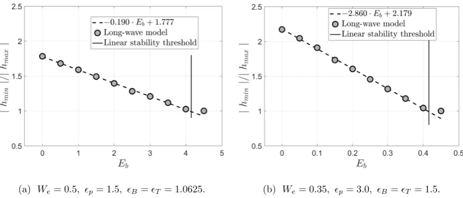
The nonlinear computations extend toO(103−104) time units, which enables further insight into the long term dynamics of the system. Quantifying the regularization of the interfacial shapes as a function of the electric field strength is best illustrated by considering the aspect ratios χof the saturated profiles, which are extracted from the final time of each computation. At this stage all maxima are within 10−2 of the wall and going beyond this minimum thickness requires prohibitively long computations. Fig. 6 illustrates the ratio χ = |hmin|/|hmax| as a function of Eb for both example cases discussed up to this point. The same salient feature is
observed in both scenarios, namely that up to the point at which Eb is sufficiently large to
stabilize the flow, the aspect ratios vary linearly withEb; the final profiles used to extract these
(a) We= 0.5, p= 1.5, B=T = 1.0625. (b) We= 0.35, p= 3.0, B=T = 1.5.
FIG. 6. Aspect ratio as a function of the electric field strength for the saturated profiles.
which corresponds to a regular cosine shape when Eb is large enough to be close to its complete
stabilization value. The negative slope varies depending on the remaining parameters We, p,
B, T; however once a critical value of Eb is reached (close to the linear stability threshold), χ
becomes unity and remains so beyond the threshold.
The modification in the interfacial shape characteristics may also be understood in view of the amount of liquid contained in the primary structures of the profile. When the electric field is absent we find a large collar and a small amplitude lobe coexisting after sufficiently long times. The lobes are centered symmetrically at x = ±π and extend to x = ±a where
a < π; the interface has local maxima atx =±a. To facilitate comparisons between different computations, we consider the interfacial profiles at final times when 1−hmax <0.01, i.e. the
interface is at a distance of 0.01 from the wall. Using this condition we find that when Eb = 0
the lobe edges are at the coordinates ±2.24. The main collar formed between these points contains 98.77% of the total liquid in the film, with the remaining small quantity shared by the secondary lobes.
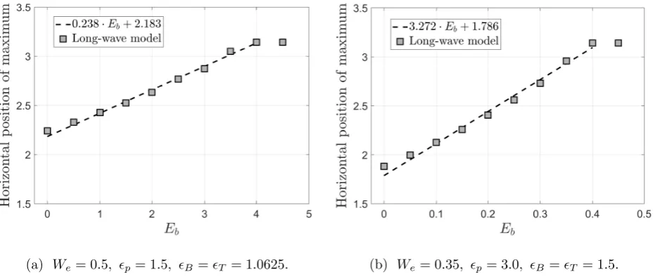
As the electric field strength is increased the lobe edge coordinates move towards the domain edges. This is illustrated in Fig. 7(a) for case a) and up the valueEb = 4.0 when the stabilizing
action of the non-zero voltage prevents lobe formation. In general, an increase in Eb reduces
the volume of the secondary lobes; these disappear completely and all the liquid is in the main collar beyond a certain threshold value of Eb. The second parameter study for case b)
reveals a similar behavior, with anticipated quantitative differences. Fig. 7(b) indicates a more pronounced displacement of the maxima, with the secondary lobes being more prominent for smaller values ofEb. Less than 94.24% of the liquid lies inside the main collar when no voltage
(a) We= 0.5, p= 1.5, B=T = 1.0625. (b) We= 0.35, p= 3.0, B=T = 1.5.
FIG. 7. The interfacial maxima horizontal coordinate considered in absolute value as the distance
from the origin atx= 0 in a domain of size [−π, π] for (a)We= 0.5, p= 1.5, B=T = 1.0625 and
(b) We = 0.35, p = 3.0, B =T = 1.5. All data has been extracted at the timestep at which the
interfacial maxima first approach the upper wall to within a distance of less than 0.01.
surface tension. When Eb ≥0.4, the secondary lobe disappears with the liquid draining inside
a single collar occupying the entire horizontal extent of the domain.
(a) Distance from wall of hmax(t). (b) Draining rate.
FIG. 8. Asymptotic behavior of the interfacial maximum hmax as the interface approaches the wall
forWe= 0.5, p = 1.5, B=T = 1.0625 and a selection of electric field strength valuesEb.
Finally we consider the draining rate of the fluid which is the rate at which the interfacial maximum approaches the wall. In accord with the similarity solutions of [21] and [4], and also in good agreement to the more recent exploration of [5], we find this rate to be (1−hmax)∝t−1/2;
[image:16.595.67.534.427.619.2]to reach this rate increases with Eb, we find that for all values of Eb tested where instability
is supported, the algebraic thinning rate follows the 1/2 power law, thus suggesting that the electric field does not enter into the dominant asymptotic balances.
IV. DIRECT NUMERICAL SIMULATIONS
To complement our asymptotic study and to further explore the dynamics in the fully non-linear non-slender regime, we carry out direct numerical simulations of the problem using the volume-of-fluid software
Gerris
([22],[23]). The second-order accuracy in both time and space of the finite volume formulation, coupled with computational capabilities such as adaptive mesh refinement (AMR) and parallelization features, all contribute to a highly efficient numerical methodology. We refer the interested reader to our previous work [18] for an outline of relevant numerical aspects in the context of a related electrohydrodynamical problem.IV.1. Methodology
A sketch of the problem has been given in Fig. 1. In the direct numerical simulations the action of the lower and upper solids is retained and these are modeled as highly dense and viscous fluids. In addition, the associated surface tension between fluids 0 and 1, as well as 2 and 3, is taken to be large. The bottom and top layers emulate the effects of solids playing a passive role in the fluid dynamical solution, with only the electric problem being of interest there. The direct numerical simulation (DNS) setup is two-dimensional and all fluids are considered to be incompressible, immiscible and viscous. They are also considered to be perfect dielectrics.
A different non-dimensionalization procedure is followed for the DNS in order to improve the stability of the discretization scheme involved. In what follows stars are used to denote dimensional quantities. The governing equations are the Navier-Stokes equations (1) and the Laplace equation for the voltage potentials (3), where it is understood that these now hold in each domain 0,1,2 and 3. Electric contributions appear in the form of jumps at the interface in the Maxwell stresses in the appropriate terms of the normal stress balance - see [18] for details on how these are incorporated as source terms in the momentum equations.
We use the horizontal length of the channel L∗D as reference length and U∗ = pg∗L∗
D as
reference velocity. With the exception of permittivity, the physical properties of fluid 2 are used as reference, and pressures are scaled byρ∗2U∗2. The permittivities are scaled with respect to the values in fluid 1. There are four main dimensionless groups arising:
˜
g = g ∗L∗
D
U∗2 ≡1, µ˜ =
µ∗2 ρ∗2pg∗L∗
DL
∗
D
, σ = σ
∗ 12
ρ∗ 2g∗L∗D2
, Eb =
∗1V∗2 0
ρ∗ 2g∗L∗D3
The quantity ˜g represents an inverse squared Froude number and setting it to 1 allows us to recover a suitable reference velocity; ˜µis an inverse Reynolds number acting as dimensionless viscosity.; an inverse Weber numberσ acts as dimensionless surface tension. The dimensionless electric field group Eb is set to 1 in and provides a reference voltage in the system given by
V0∗ = pρ∗2g∗L∗3
D/
∗
1. The quantity ¯V = ¯V ∗/V∗
0 (note that the electric field is E
∗ = ¯V∗/L∗
D)
measures the magnitude of the applied voltage potential difference. For notational convenience we introduce the following physical property ratios:
r0 =ρ∗2/ρ ∗
0, r1 =ρ∗2/ρ ∗
1, r3 =ρ∗2/ρ ∗
3, m0 =µ∗0/µ ∗
2, m1 =µ∗1/µ ∗
2, m3 =µ∗3/µ ∗
2, (45)
B =∗0/ ∗
1, T =∗3/ ∗
1, p =∗2/ ∗
1, s10= (σ∗10/σ ∗
12)σ, s32= (σ∗32/σ ∗
12)σ. (46) The quantities σ∗10, σ12∗ and σ∗32 denote the surface tension coefficients between the fluids in regions 1 and 0, 1 and 2, 3 and 2, respectively. The dimensionless domain has unit horizontal extent and lies in −1/2 < x < 1/2. For the hydrodynamics at the end points x = ±1/2 we impose impermeability u(±1/2, y, t) = 0 and free-slip vy(±1/2, y, t) = 0. A voltage potential
difference ¯V is maintained by prescribing a non-zero voltageφ
x=−1/2 = ¯V on the left boundary, with φ
x=+1/2 = 0 on the right. The dimensionless liquid layer region 2 has mean thickness while region 1 lying below it has dimensionless mean thickness 21π. The bounding slab regions 0 and 3 are taken to have a finite vertical thickness of dimensionless sizeL0 = 12(1−−21π), rather than the semi-infinite extent employed in the analysis. More specifically in their undisturbed states, region 0 occupies −1
2 < y <− 1
2 +L0, region 1 occupies − 1
2 +L0 < y <− 1
2 +L0+ 1 2π =
1 4π −
2, region 2 occupies 1 4π −
2 < y < 1 4π +
2, and region 3 occupies 1 4π +
2 < y < 1 2. At the outer walls y= −1
2 and y = 1
2 we impose no-slip conditions u =v = 0 and a zero vertical electric field component ∂yφ0(x,−1/2, t) = 0 and ∂yφ3(x,1/2, t) = 0. Note that while in the asymptotic model regions 0 and 3 are considered to be semi-infinite, we found that imposing a wall at a finite distanceL0 away has inconsequential effects on the flow; furthermore numerical experiments showed that L0 = O(10−1) is sufficient. For completeness the schematic of the domain utilized in the DNS is included in Fig. 9.
A sinusoidal initial perturbation of the fluid interface y=h(x, t) is imposed
h(x,0) =−Acos(2πqx), (47)
FIG. 9. Schematic of the computational domain utilized in the direct numerical simulations.
IV.2. Comparison of DNS with thin film model results
Recall that the solutions of the evolution equation (41) depend on five dimensionless physical parameters, the surface tension parameterWe, the electric field strengthEband the permittivity
ratios B, T and p. The thin liquid layer assumption, along with the passive nature of the
fluid in region 1, enabled analytical progress and derivation of a tractable partial differential equation which retains desired physical effects. By contrast, the direct numerical simulations employing the volume-of-fluid methodology introduce additional complexity. Firstly, the small liquid layer height 1 was scaled out of the analysis, however a suitable choice is required when modeling the full two-dimensional computational domain. It is anticipated that if
on the interfacial shape and other nonlinear features. Finally, concrete choices must be made for the density ratios r0, r1 and r3, and the viscosity ratios m0, m1 and m3, so that the fluid system is Rayleigh-Taylor unstable and the contrast in physical quantities is sufficiently strong to reflect the idealized configuration of an upper liquid layer with a passive fluid underneath.
The challenges described above render a one-to-one correspondence with the asymptotic solutions very difficult to attain. Furthermore, the DNS are made even more expensive due to the slow timescale of the flow for small and as wall touching takes place. Resolving such layer thinning dynamics for the model equation required O(103−104) time units (see Fig. 8). Noting the −3 rescaling in the time variable - see equation (26) - and the smallness of , it is anticipated that the number of time units needed to observe the same features in the DNS will increase prohibitively by a factor of at least 103forsmaller than 0.1. Two simplifications, that arose from extensive numerical experimentation, were introduced to surmount these difficulties. The value for has been set to 0.2L = 0.2/(2π), which was found to be sufficiently small to reproduce the findings of the model. Secondly, the Reynolds number used in the computations has been increased by a factor of approximately three, so that when re-cast into the non-dimensionalization (44), its inverse becomes ˜µ = 0.02 instead of 0.0635 which would directly coincide with Re = 1 used in the model. These parameter choices accelerate the computations significantly and provide results from direct numerical simulations that can be compared with the asymptotic model solutions. Adaptive grid refinement is used, which is set to increase resolution in the vicinity of the interface and the thin liquid layer. Adaptivity allows for coarser grids away from the thin layer but a large number of degrees of freedoms emerge still. For example, prescribing the highest level of refinement around the interface to be 256 cells, adaptivity yields approximately 5·103 degrees of freedom; this is an order of magnitude less than what it would be over a uniform grid at the resolution of the interface. Nonetheless, to capture the dynamics of the interface as it gets close to the wall we require at least 1000 CPU hours for each run.
For the first test case we take a surface tension coefficient σ = 0.012665 and permittivity ratios p = 1.5 and B = T = 1.0625, all being equivalent to the values used in the study
of the long-wave model in subsection III. The imposed voltage potential difference ¯V varies from 0.0 to 0.46, with the threshold for instability for a wavenumber of 2π is found to be of
¯
contribution. The second test case is characterized by σ = 0.008865, p = 3.0, B = T = 1.5
and ¯V varying from 0.0 to 0.235, with s10 = s32 = 56.5. The remaining physical parameters pertaining to the direct numerical simulations in both studies are density ratios r0 = 1.0,
[image:21.595.67.533.171.401.2]r1 = 80.0, r3 = 10.0, viscosity ratios m0 = 5.0, m1 = 1.0, m3 = 1.0 and inverse Reynolds number ˜µ= 0.02.
FIG. 10. Evolution of maximumhmax(t) and minimumhmin(t) positions of the interface in time for
σ = 0.012665, p = 1.5, B = T = 1.0625 and varying ¯V. The remaining physical parameters for
the DNS are ˜µ = 0.02, s10 = s32 = 39.47, r0 = 1.0, r1 = 80.0, r3 = 10.0, m0 = 5.0, m1 = 1.0 and
m3 = 1.0.
The time evolution of the scaled interfacial maximum and minimum are depicted in Fig. 10, to be compared to the analogous Fig. 3 in the asymptotic study. To enable comparisons with the model computations, the interfacial position for the DNS is written ash(x, t) = 41π−
2+˜h(x, t) and hence the scaled interface is ˜h(x, t) = (h(x, t)− 1
4π +
introduced by the initial condition.
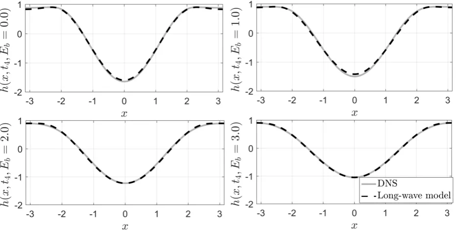
FIG. 11. Interfacial shape comparison as hmax = 0.9 for increasing values of Eb (dots labeled t4 of Fig. 3 for the long-wave model) and ¯V (dots labeledt4 of Fig. 10 for the direct numerical simulations)
for the first choice of parameters -σ = 0.012665, p = 1.5, B =T = 1.0625. Top left Eb = 0.0, top
right Eb= 1.0, bottom left Eb = 2.0, bottom rightEb = 3.0.
FIG. 12. Interfacial shape comparison ashmax= 0.9 for increasing values ofEb and ¯V for the second
choice of parameters -σ = 0.008865, p = 3.0, B =T = 1.5. Top leftEb = 0.0, top right Eb = 0.1,
[image:22.595.70.536.464.704.2]The shapes of the interface obtained from the DNS are compared to their counterparts from the long-wave model in Fig. 11 and Fig. 12 for the two different cases investigated. The four panels show the superimposed interfaces when hmax first exceeds 0.9, indicated by circles in
Fig. 3 and Fig. 10. Excellent agreement is found between long-wave and DNS results, with the nonlinearity in the shape being regularized to a cosine shape as the electric field is increased. More pronounced features are observed in the second case due to a smaller value of σ. For values of the field near the stabilization threshold, our results indicate that nonlinear distortion is reduced and the shapes grow towards the wall retaining their initially sinusoidal profiles.
[image:23.595.66.531.237.431.2](a) σ= 0.012655, p= 1.5, B=T = 1.0625. (b) σ= 0.008865, p= 3.0, B=T = 1.5.
FIG. 13. Aspect ratio as a function of the electric field strength for the saturated profiles based on
results originating from the direct numerical simulations.
The dependence between the interfacial shape aspect ratioχ=|hmin|/|hmax|as a function of the electric field strength is summarized in Fig. 13. Given the linear dependence ofχtoEb once
saturation is reached in the long-wave model (see Fig. 6), we anticipate a similar behavior in the DNS. Noting that ¯V ∼√Eb with Eb defined by (10), we expect a linear variation ofχ with
¯
(results not shown) that when we increase the vertical extent of the lower side of the domain and remove the lower fluid from the system, dripping can occur should exceed a threshold value for a given ¯V.
IV.3. Using DNS to test the validity of the long-wave equations
[image:24.595.69.538.392.633.2]Even though the evolution equation (41) is valid for 1, the numerical simulations of section IV.2 have shown that agreement is excellent for = 0.2/(2π). In what follows we examine numerically the solution dependence on the liquid film height and characterize the dynamics at progressively larger values of in order to evaluate the validity of the model (41). In order to reduce the number of parameters we concentrate on the non-electrified case ¯V = 0. We take parameters similar to those of the first case described in subsection IV.2, with density ratios r0 = 1.0, r1 = 80.0, r3 = 10.0, viscosity ratios m0 = 5.0, m1 = m3 = 1.0 and surface tension coefficient σ = 0.012665, while s10 = s32 = 39.47 (permittivity ratios are no longer relevant). In order to promote a shorter timescale of the dynamics for the smaller values of , the dimensionless viscosity is reduced to ˜µ= 0.001.
FIG. 14. Evolution in time of the scaled maximum hmax(t) and minimum hmin(t) positions of the
interface as the liquid film height is increased.
Fig. 14 presents results for varying between (0.1/2π) and (0.49/2π). Here we plot the interfacial extrema hmax and hmin for all test cases, normalizing each by the appropriate value of 2πi, i= 1, . . . ,11 - as previously, this normalization implies that the interface touches the
and so its normalized value varies appropriately. We find that larger values ofpromote a faster growth of the instability, while the added fluid mass also affects interfacial shapes sufficiently close to the upper wall. More specifically, by plotting interfacial shapes as they first reach the maximum value ofy= 0.9 (circles att4in Fig. 14), we find that the increase in fluid mass pushes the maxima further inward in the domain, supporting a stronger deformation of the interface at its minimum point where x = 0.0 - see Fig. 15(a). This resembles the effect obtained when reducing the surface tension coefficient in the comparison between the two different cases analyzed previously. Quantifying the shape aspect ratio χ = |hmin|/|hmax| once the shapes have saturated, shows a significant increase in the nonlinearity with χ changing from 1.78 for the smallest value of = (0.1/2π) to almost 2.4 as reaches values closer to (0.5/2π) - see Fig. 15(b). Values of 2π ≤ 0.25 are estimated to be in good agreement (errors of less than 5%) with the asymptotic model based on this property.
[image:25.595.65.531.323.494.2](a) Scaled interfacial shapes ashmax= 0.9. (b) Aspect ratio of scaled saturated shapes.
FIG. 15. Interfacial shape properties as a function of varying liquid film height.
FIG. 16. Pressure field for a large = (0.49/2π) case with a close-up of the region where the active
fluid interface approaches the lower fluid layer and a thin region (cushion) is created between them.
Beyond this stage the fluid simply extends laterally.
[image:25.595.80.515.577.653.2]mesh refinement illustrated in the figure, ensures that such dynamics is computed accurately even as the thickness of this intermediate layer becomes very small. At this stage the upper liquid layer effectively rests on the lower surface; further increases in lead to the lateral spreading of the upper liquid on top of this (slightly compliant) surface. We note that as a result of the modeling, a small level of deformation of the lower interface is present. Further increases in the viscosity, density and surface tension coefficient in the lower passive layer would alleviate this artifact, however the deformation is found to be sufficiently small to have a negligible effect on the overall dynamics of the system.
The results presented indicate that the asymptotic model captures the main features of the flow well even for relatively large values of . Qualitatively there are only minor modifications in the flow even until the lower surface is reached, while quantitatively we find good agreement between the results based on the long-wave evolution equations and the DNS for 2π≤0.25.
The results thus far consider systems with relatively strong surface tension that are confined from below, and hence pendant drop formation, elongation and subsequent dripping have not been observed. We have investigated such phenomena (details omitted here for brevity) by removing the lower fluid 0 and extending region 1 vertically so that bottom wall effects become negligible; all other parameters described earlier in this subsection are kept fixed. We find that for ≤ 0.4, the results coincide with the confined case. When ≈ 0.45, minor differences emerge as the liquid layer interacts with the lower interface when the latter is present. As
exceeds a value of approximately 0.5 the formation of a pendant drop and eventual dripping is observed - pinching can only happen if additional effects such as van der Waals forces are included. It is useful to compare the critical value of found for dripping, with the capillary length`c=
p
σ∗12/(ρ∗2g∗). Taking layer 1 to be air, i.e. ρ∗
1 ≈1.225kg/m3 and taking parameters as in the DNS performed in this section, we have the density of the liquid layer region 2 being
ρ∗2 =r1ρ∗1 ≈98kg/m3. In addition, assuming a surface tension coefficient σ ∗
12 = 72·10
−3N/m
(this is a typical value for water-air interfaces), we find `c ≈ 8.6mm. The value of L∗D can
be found from the dimensionless surface tension formula σ = (σ∗12/ρ∗2g∗L∗2
D) which was set to
σ = 0.012665 in the present computations. We findLD ≈7.7cm, and since the critical value of
V. APPLICATION: ACTIVE CONTROL OF THE RAYLEIGH-TAYLOR
INSTABIL-ITY
In what follows we use a time-dependent electric field to produce controlled interfacial oscil-lations, with no moving mechanical parts, with possible implications for mixing at small scales. Simple control protocols have already been investigated in a geometry of infinite vertical extent [18] and then tailored towards mixing studies in two and three dimensions [24] when the walls were placed far away from the undisturbed position of the interface. The latter study uses vertical electric fields to introduce instability in otherwise stably stratified flows; here we use horizontal electric fields to arrest gravitational instabilities. Results using both the long-wave model and DNS will be presented.
To fix matters we solve the evolution equation (41) with the same parameters as in case b) in section III, i.e. We = 0.35, p = 3.0 and B = T = 1.5. The electric field strength Eb
is chosen to alternate between 0 and 0.75, which is above the stability threshold predicted by linear theory and is selected to induce stabilization even when outside the linear regime.
(a) Evolution of interfacial minimumhminand
maximumhmax in time.
(b) Interfacial shapes immediately prior to switching
[image:27.595.177.516.386.549.2]on the electric field in four different cycles.
FIG. 17. On-off electric field with the electric field activated when hmax exceeds the threshold value
yt= 0.5 and switched off when the interface maximum reaches the same level as in the initial condition.
The suggested mechanism is summarized as follows. Starting from a k = 1 initial pertur-bation and an initial amplitude of 5·10−4, we allow the Rayleigh-Taylor instability to evolve naturally until a certain threshold level yt is reached by the interfacial maximum hmax(t). As soon as yt is exceeded, the electric field is switched on and, after an initial transient, a strong
initial amplitude, and repeat this cycle over several periods.
Fig. 17(a) shows the evolution of the interfacial extrema hmin(t) (dashed curve) andhmax(t) (solid curve) over the duration of the nonlinear calculation. The background is colored in white when the electric field is switched off, allowing the instability to grow over tens of time units. Once hmax reaches the threshold level, the electric field is switched on as illustrated with a dark gray background. Under the stabilizing action of the field, both extrema decrease to their initial amplitudes as seen in the Fig. 17(a). A threshold valueyt= 0.5 is sufficient for nonlinear
effects to emerge, and Fig. 17(b) presents the interfacial shapes one time-step before the electric field is switched on. The results strongly suggest a robust time-periodicity of the phenomena. The duration of the periods when the field is off is toff ≈ 36.26, while the on-periods are slightly smaller with ton ≈32.7. The interfacial shapes are virtually indistinguishable between consecutive on-off cycles. The robustness of the dynamics suggests that we can repeat the oscillations over several tens or hundreds of cycles to reach competitive mixing designs. We also note that even though a time-dependent electric field is proposed in the context of a quasi-static approximation, the scales involved ensure the validity of such an approach (see Appendix B of [18] for details).
(a) Interface maximum as a function of time for different values of ¯V when
switching the electric field on att= 245.5 (single cycle).
(b) hmin(t) andhmax(t)
[image:28.595.61.538.404.641.2]evolution.
FIG. 18. On-off electric field with the electric field activated when hmax exceeds the threshold value
yt= 0.5 and switched off when the interface maximum reaches the same level as in the initial condition.
The evolution of the interfacial extremahmax(t) andhmin(t) is compared to the dynamics obtained in
the equivalent configuration in the long-wave model, presented previously in Fig. 17(a).
We use the same parameter values as in the second test case in subsection IV.2. For the parameters of Fig. 17(a)-17(b), the equivalent stabilizing voltage to be imposed is ¯V ≈ 0.3. Results with a number of different values of ¯V are illustrated in Fig. 18(a); it can be seen that voltages ¯V >0.25 stabilize the interface and return it to its almost flat state by the end of the computation. For values of ¯V ≈0.3 the relative duration of off- and on-cycles as well as shapes are in good agreement between the long-wave model and the DNS.
Next we turn to a more stringent threshold yt = 0.9 that allows the interface to get closer
to the wall before the field is turned on to cause stabilization and sustained oscillations. We proceed with computations based on the model (41) due to the prohibitive cost of the DNS in this case. Figures 19(a) and 19(b) indicate that once again the on-off cycles are sustained robustly even in this more challenging regime. Here the off-periods increase from 36.25 time units to approximately 85.64 time units in order to accommodate the growth closer to the wall. By comparison, the on-periods only require a mild increase in order to steer the interface back to its initial perturbation.
(a) Evolution of interfacial minimumhminand
maximumhmax in time.
(b) Interfacial shapes immediately prior to switching
[image:29.595.51.523.358.581.2]on the electric field in four different cycles.
FIG. 19. On-off electric field with the electric field activated when hmax exceeds the threshold value
yt= 0.9 and switched off when the interface maximum reaches the same level as in the initial condition.
VI. CONCLUSIONS
coupling with the fluids inside the channel. The analysis leading to equation (41) was carried out for bounding slabs of infinite extent, and this is appropriate since the channel thickness is typically smaller than that of the slabs. The theory can be modified in a straightforward way for slabs of finite thickness, at the expense of more complicated Fourier symbols of the non-local term in (41). In addition, direct numerical simulations that necessarily use finite slab geometries, were found to be in excellent agreement with the model. We also demonstrated the possibility of using the imposed electric field as an active control parameter to induce sus-tained time-periodic nonlinear oscillations of the interface that may have relevance in mixing in small-scale geometries - see [24] for related approaches.
There are several research directions that can be pursued based on this work, including the effect of topographical structures (e.g. of finite extent for simplicity) on the wall wetted by the liquid layer as well as the addition of pressure-driven flow as encountered in microfluidic devices, for instance. In the former case the effect of wall topography will induce a non-uniform field locally and hence non-uniform base states as opposed to the flat ones studied here. Adding flow coupled with horizontal field stabilization is expected to produce active-dissipative dynamics reminiscent of the Kuramoto-Sivashinsky equation, for example.
ACKNOWLEDGMENTS
The work of RC and DTP was supported by the Engineering and Physical Sciences Research Council (EPSRC) under grants EP/K041134/1 and EP/L020564/1.
Appendix A: Numerical method for the thin-film equation
We consider the problem of numerically solving (41) in the form
Ht+ [f1(H)Hxxx]x+ [f2(H)]xx+ [f3(H)(B[H](x))xx]x = 0, (A1)
where B[H](x) is the non-local term due to the electric field known in Fourier space as (40), and the polynomial functions fi(H);i= 1,2,3 are as follows
f1(H) =
W e
3 (1−H) 3, f
2(H) =− 1
12(1−H) 4, f
3(H) =
Eb(1−p)
3 (1−H)
3, (A2)
by discretizing it on a periodic domain x ∈ [−L, L] using the finite difference method pre-sented in [20] and modified as described below in order to include the new electric field term, [(f3(H)B[H](x))xx]x.
We first briefly describe the discretization of the fluid part (Eb = 0) of (A1) with second-order
Using the convention xm+1/2 = (xm +xm+1)/2, we obtain the following system of ordinary
differential equations
dHm
dt +
f1(Hm+1/2)∂3(H)m+1/2−f1(Hm−1/2)∂3(H)m−1/2
∆x +∂2(f2(H))m = 0, (A3)
where we note that ∂i represents a standard second-order accurate finite difference
approxi-mation to the ith spatial derivative. The ODE system (A3) is discretized in time with the second-order accurate Crank-Nicolson scheme as
Hn+1+ ∆t 2 F
fluid(Hn+1) = Hn− ∆t
2 F
fluid(Hn). (A4)
and, at every time step, we solve a nonlinear algebraic system for Hn+1 with Newton iteration for which the Jacobian matrix is
J=I+∆t
2
∂Ffluid
∂H , (A5)
where the elements of the ∂F∂fluidH matrix are known explicitly.
Next, our modification of the scheme in [20] is described by considering the following evolu-tion PDE
Ht+ [f3(H)(B[H](x))xx]x = 0, (A6)
with periodic boundary conditions. We let Hn be the discretization of H at time t
n on the
computational grid. The Crank-Nicolson discretization in time is then, using the product rule,
Hn+1−Hn
∆t +
1 2[f
0
3(h)(DxH)Bxx+f3(H)Bxxx] n+1
+1 2[f
0
3(H)(DxH)Bxx+f3(H)Bxxx] n
= 0,
where the vector-vector products are computed point-wise, and the Dx operator is the discrete
differentiation operator. We now need a method for calculating the Jacobian of the function evaluations and we cannot use the FFT to compute the non-local term. We thus rewrite the equation above in the following way
Hn+1+∆t 2
h
f30(H)(DH)(GH) +f3(H)( ˜GH) in+1
=−∆t
2 h
f30(H)(DH)(GH) +f3(H)( ˜GH) in
,
where we made the operator substitutions in notation: Dx =:D, Bxx =:GH,Bxxx =: ˜GH. We
identify the bracketed term in the left-hand side of the above equation with Felectric(Hn+1), and see that we now have a nonlinear system of equations to solve, and need an explicit formula
for ∂Felectric∂H to perform Newton iteration. To this end we denote the discrete Fourier transform
matrix as MF, k is the wavenumber, and write out our operators in matrix form as
G:=M−F1Σ1MF, Σ1 := diag(−k2λ(k)),
D:=M−F1Σ2MF, Σ2 := diag(ikλ(k)), ˜
G:=M−F1Σ3MF, Σ3 := diag(−ik3λ(k)),
and define di, gi, and ˜gi as the i-th row of D,G,G˜ respectively, where
λ(k) =i(1−p)
kcosh(k) +B|k|sinh(k)
(B+T)|k|cosh(k) + (1 +BT)ksinh(k)
(A8)
is the symbol in Fourier space of the convolution kernel deduced from (40). Using this notation we derive the following relationships for the elements of the Jacobian, J.
m6=j : ∂F electric
m
∂Hj
= ∆t 2 (f
0
3(Hm)Dmj(gm·H) +f30(hm)(dm·H)Gmj +f3(Hm) ˜Gmj),
m=j : ∂F electric
m
∂Hj
= 1 +∆t 2 (f
00
3(Hm)(dm·H)(gm·H) +f30(hm)Dmj(gm·H)
+f30(Hm)(dm·H)Gmj +f30(Hm)(˜gm·H) +f3(Hm) ˜Gmj).
(A9)
Adding the matrix (A9) to the ∂F∂fluidH matrix allows us to perform Newton iterations to solve for Hn+1 in the presence of both the fluid and the electric field terms.
In our implementation we refine the spatial grid whenever a finer discretization is detected to be required in order to accurately resolve finer features of the evolving solution. Specifically, we take a Fourier transform of the solution in each time step and examine the magnitudes of the Fourier modes. When more than a threshold, for example, 23 of the Fourier modes are larger than a tolerancex we double the number of grid points. Note that this implies we are implementing
global adaptivity, not adaptivity only in regions with finer features. Implementing our upscaling method is straightforward with Fourier interpolation; we take our Fourier transformed solution ˆ
hM on a grid with M gridpoints, pad M higher wavenumbers with zero, and then transform
back to obtain a solution h2M defined on 2M gridpoints. We also control the timestep by
employing a local error indicator em which approximates ∆Htn−1n m
d2Hn m
dt2 [20, 25]:
em =
2∆tn−1 ∆tn−2
∆tn−2Hmn+1+ ∆tn−1Hmn−1−(∆tn−2+ ∆tn−1)Hmn
(∆tn−2+ ∆tn−1)Hmn
. (A10)
We increase ∆t by 10% whenever em < 34t for all m and decrease it when em > t, where et is
the time accuracy to be maintained throughout the computation time interval. For solving the linear systems in the nonlinear Newton iterations, we additionally use a GMRES solver with a preconditioner derived from the linearized form of equation (A1) [26].
[1] S.G. Yiantsios and B.G. Higgins, “Rayleigh-Taylor instability in thin viscous films,” Physics of
Fluids A 1, 1481–1501 (1989).
[2] L.A. Newhouse and C. Pozrikidis, “The Rayleigh-Taylor instability of a viscous liquid layer resting
[3] A. Egowainy and N. Ashgriz, “The Rayleigh-Taylor instability of viscous fluid layers,” Physics
of Fluids 9, 1635–1649 (1997).
[4] P.S. Hammond, “Nonlinear adjustment of a thin annular film of viscous fluid surrounding a thread
of another within a circular cylindrical pipe,” Journal of Fluid Mechanics 137, 363–384 (1983).
[5] J.R. Lister, J.M. Rallison, A.A. King, L.J. Cummings, and O.E. Jensen, “Capillary drainage of
an annular film: the dynamics of collars and lobes,” Journal of Fluid Mechanics 552, 311–343
(2006).
[6] L. Limat, P. Jenffer, B. Dagens, M. Fermigier, and J.E. Wesfreid, “Gravitational instabilities of
thin liquid layers: dynamics of pattern selection,” Physica D 61, 349–383 (1992).
[7] M. Fermigier, L. Limat, J.E. Wesfreid, P. Boudinet, and C. Quillet, “Two-dimensional patterns
in Rayleigh-Taylor instability of a thin layer,” Journal of Fluid Mechanics 236, 349–383 (1992).
[8] J.R. Lister, J.M. Rallison, and Rees S.J., “The nonlinear dynamics of pendent drops on a thin
film coating the underside of a ceiling,” Journal of Fluid Mechanics 647, 239–264 (2010).
[9] A.J. Babchin, A.L. Frenkel, B.G. Levich, and G.I. Sivashinsky, “Nonlinear saturation of
Rayleigh-Taylor instability in thin films,” Physics of Fluids 26, 3159–3161 (1983).
[10] D. Halpern and A.L. Frenkel, “Saturated Rayleigh-Taylor instability of an oscillating couette film
flow,” Journal of Fluid Mechanics 446, 67–93 (2001).
[11] O. Haimovich and A. Oron, “Nonlinear dynamics of a thin liquid film on an axially oscillating
cylindrical surface,” Physics of Fluids (1994-present) 22, 032101 (2010).
[12] J.R. Melcher, “Electrohydrodynamic and magnetohydrodynamic surface waves and instability,”
Physics of Fluids 4, 1348–1354 (1961).
[13] J.R. Melcher,Field-Coupled Surface Waves (Technology Press, Cambridge, Massachusetts, 1963).
[14] N.T. Eldabe, “Effect of a tangential electric field on Rayleigh-Taylor instability,” J. Phys. Soc.
Japan 58, 115–120 (1989).
[15] A. Joshi, M.C. Radhakrishna, and N. Rudraiah, “Rayleigh-Taylor instability in dielectric fluids,”
Physics of Fluids (1994-present) 22, 064102 (2010).
[16] L.L. Barannyk, D.T. Papageorgiou, and P.G. Petropoulos, “Supression of Rayleigh-Taylor
in-stability using electric fields,” Mathematics and Computers in Simulation82, 1008–1016 (2010).
[17] L.L. Barannyk, D.T. Papageorgiou, P.G. Petropoulos, and J.-M. Vanden-Broeck, “Nonlinear
dynamics and wall touch-up in unstably stratified multilayer flows under the action of electric
fields,” SIAM Journal on Applied Mathematics 75, 92–113 (2015).
[18] R. Cimpeanu, D.T. Papageorgiou, and P.G. Petropoulos, “On the control and suppression of
the Rayleigh-Taylor instability using electric fields,” Physics of Fluids (1994-present)26, 022105
[19] D.T. Papageorgiou and J.-M. Vanden-Broeck, “Large-amplitude capillary waves in electrified fluid
sheets,” Journal of Fluid Mechanics 508, 71–88 (2004).
[20] D. Tseluiko and D.T. Papageorgiou, “Nonlinear dynamics of electrified thin liquid films,” SIAM
Journal on Applied Mathematics 67, 1310–1329 (2007).
[21] A.F. Jones and S.D.R. Wilson, “The film drainage problem in droplet coalescence,” Journal of
Fluid Mechanics 87, 263–288 (1978).
[22] S. Popinet, “Gerris: A tree-based adaptive solver for the incompressible Euler equations in
com-plex geometries,” J. Comput. Phys. 190, 572 (2003).
[23] S. Popinet, “An accurate adaptive solver for surface-tension-driven interfacial flows,” J. Comput.
Phys. 228, 5838 (2009).
[24] R. Cimpeanu and D.T. Papageorgiou, “Electrostatically induced mixing in confined stratified
multi-fluid systems,” Int. J. Multiphase Flow 75, 194–204 (2015).
[25] A.L. Bertozzi and M. Pugh, “The lubrication approximation for thin viscous films: the moving
contact line with a ’porous media’ cut-off of van der Waals interactions,” Nonlinearity 7, 1535
(1994).
[26] L.S. Mulholland and D.M. Sloan, “The role of preconditioning in the solution of evolutionary
par-tial differenpar-tial equations by implicit Fourier pseudospectral methods,” Journal of Computational