Testing for Speculative Bubbles using Spot and Forward
Prices
∗Efthymios G. Pavlidis†, Ivan Paya, and David A. Peel
Department of Economics, Lancaster University Management School, UK
Abstract
The probabilistic structure of periodically collapsing bubbles creates a gap be-tween future spot and forward (or futures) asset prices in small samples. By ex-ploiting this fact, we use two econometric methods, namely, the recursive unit root method of Phillips, Shi, and Yu (2015a,b) and the rolling regression method of Fama (1984), for detecting bubbles. Both methods do not rely on a particular model of asset price determination, they are robust to an explosive root in the process for market fundamentals, and are accompanied by a date-stamping strategy. By ap-plying these methods to the German mark-US dollar and British pound-US dollar exchange rates, we provide evidence in favor of speculative bubbles in the foreign exchange market during the interwar German hyperinflation, but not during the recent floating-rate period. A further application to the S&P 500 index supports the existence of speculative bubbles in the US equity market.
Keywords: Rational bubbles, Forward exchange rates, Futures prices, Explosive root, Hyperinflation.
JEL Classification: C12, C22, F31.
∗For comments and suggestions, we are grateful to the editor, two anonymous referees, Karim Abadir,
Mehmet Caner, Tom Engsted, Atshushi Inoue, Bruce Mizrach, Bent Nielsen, Garry Phillips, Peter C. B.
Phillips, Phil Rothman, Michalis Stamatogiannis, Mike Tsionas, and participants of the 5thCSDA
Inter-national Conference on Computational and Financial Econometrics, the 19thAnnual Symposium of the
Society for Nonlinear Dynamics and Econometrics, the 2015 Annual Conference of the Royal Economic So-ciety, the North Carolina State University Econometrics Workshop, the Workshop on Recent Developments in Econometric Analysis, the University of Liverpool, the Federal Reserve Bank of Dallas, and the Bank of England. Documentation about the data used in this paper is available from the Lancaster University data
archive athttp://dx.doi.org/10.17635/lancaster/researchdata/81.
†Correspondence to: Efthymios G. Pavlidis, Department of Economics, Lancaster University
1 Introduction
A rational bubble reflects a self-confirming belief that an asset’s price depends on a vari-able (or a combination of varivari-ables) that is intrinsically irrelevant - that is, not part of market fundamentals(Diba and Grossman, 1988, p. 520). Since the widespread adop-tion of raadop-tional expectaadop-tions into macroeconomics, a large number of studies have at-tempted to empirically separate the contribution of rational bubbles and market funda-mentals to asset price movements (e.g., Balke and Wohar, 2009; Phillips et al., 2011).1 A variety of econometric tests have been developed in the literature that can be used for this purpose. The most popular include volatility, Hausman-type, and (co-)integration tests (Cochrane, 1992; Diba and Grossman, 1988; Engsted and Nielsen, 2012; LeRoy and Porter, 1981; Phillips et al., 2015a; Taylor and Peel, 1998; West, 1987, 1988).
A common feature of all tests for bubbles is that they actually examine a composite hypothesis of no bubbles and a model for market fundamentals. Because rejection of the null may be due to the presence of bubbles or model misspecification, or to both of these reasons, results are deemed to be inconclusive (Flood et al., 1994; Gürkaynak, 2008; Hamilton and Whiteman, 1985). To make matters worse, even if the specification of the true model for market fundamentals is known, econometric tests may still fail to detect bubbles if these processes periodically crash (Blanchard, 1979; Blanchard and Watson, 1983; Evans, 1991; van Norden, 1996; van Norden and Schaller, 1993). Following Evans (1991), several studies have shown that, in finite samples, periodically collapsing bubbles can make asset prices look non-explosive and co-integrated with market fundamentals, thus leading to a severe power loss of standard statistical tests.
In this paper, we propose two novel methods for detecting bubbles that periodically collapse. The methods do not rely on a particular asset price determination model, im-pose minimal assumptions on the process for market fundamentals, and, thus, alleviate the misspecification problem. The methods have two further appealing features. First, because they are recursive they allow the identification of the starting and ending points of bubble episodes. Second, they only require data on spot and forward (or futures) prices, which contrary to market fundamentals, are readily available at high frequencies and over long time periods. This latter feature is especially important in light of the low power of statistical tests (Evans, 1991; West, 1994).
Although we focus on the foreign exchange market, the methods are of general in-terest since they are applicable to any market for which spot and forward (or futures) prices are available. The underlying idea is simple: when a bubble is occurring, both the forward exchange rate and the future spot rate incorporate it but with different weights. This is due to the fact that rational agents, when forming expectations, correctly attach a
1In line with most of the empirical literature, we focus on rational extrinsic bubbles. Froot and Obstfeld
nonzero probability to the bubble bursting. As a consequence, the forward rate becomes a downward biased predictor of the future spot rate, with the difference between the two rates (i.e., the degree of the bias) depending on the bubble process and, as such, being explosive. As long as the forecast errors for fundamentals are not explosive, the presence of explosive dynamics in the difference between the two rates can be attributed to the existence of bubbles.
On this basis, rather than applying (co-)integration tests to the spot rate and a set of observed market fundamentals, which is the common practice in the literature, we advocate the application of right-tailed unit root tests to the difference between future spot and forward rates. Of the various unit root tests proposed in the literature, we em-ploy the Generalized Supremum Augmented Dickey Fuller (GSADF) recently developed by Phillips et al. (2015a). This choice is based on Monte Carlo simulation results that indicate that the GSADF exhibits good power properties in our setting.
The second method we propose is based on the failure of the unbiasedness hypothe-sis in small samples and conhypothe-sists of estimating rolling Fama regressions. The fact that the variables that enter the Fama regression are highly persistent (potentially explosive) im-plies that conventional tests may be invalid (Cavanagh et al., 1995; Engsted and Nielsen, 2012; Jansson and Moreira, 2006; Nielsen, 2010; Phillips and Magdalinos, 2008). To cir-cumvent this obstacle, we adopt the IVX instrumentation procedure of Phillips and Mag-dalinos (2009), Phillips and Lee (2013), and Kostakis et al. (2015).
We provide two empirical applications of the proposed bubble detection methods to US dollar exchange rates. In the first application, we examine one of the most stud-ied events in monetary history: the interwar German hyperinflation. The existence of speculative bubbles in hyperinflation Germany has been the subject of a considerable amount of research (see, e.g., Burmeister and Wall, 1982, 1987; Casella, 1989; Christiano, 1987; Durlauf and Hooker, 1994; Engsted, 1993, 1994; Hooker, 2000; Sargent, 1977; Tay-lor, 1991). However, no general consensus has been reached in the literature. Previ-ous studies, that focus on prices and money, find mixed results that depend crucially on the validity of a variety of different assumptions. For instance, Burmeister and Wall (1982) find that bubbles cannot be rejected if the money supply process depends on expected inflation. Casella (1989) shows that the presence of bubbles in prices can be rejected if the money supply process is assumed exogenous to current inflation but not when there is a feedback rule. Hooker (2000) shows through Monte Carlo simulations that the small sample properties of tests for bubbles may differ substantially from their asymptotic counterparts. By using finite-sample critical values, he concludes that there is evidence of misspecification in the Cagan money demand model but no evidence of bubbles. Engsted (2003) points out that Hooker’s methodology neglects the magnitude of misspecification noise in Cagan’s model. Taking the magnitude of noise into account, he also doesn’t find any evidence of bubbles.
time. Keynes, for instance, notes that foreign exchange speculation during the German hyperinflation was “on a tremendous scale and was, in fact, the greatest ever known”.2 Our results reveal two bubble episodes, one in July-August 1922, and another a year later in the summer of 1923, almost a month before forward trading was suspended by the German authorities. These two bubble periods coincide with large and persistent spec-ulative movements in the foreign exchange market (Bresciani-Turroni, 1937).
Our second empirical application focuses on the recent floating-rate period. This period is particularly interesting because, following the collapse of the Bretton Woods system, exchange rates among major currencies became volatile and highly persistent, moving in one direction over long time spans (see, e.g., Engel and Hamilton, 1990). A notable example of such movements is the large appreciation of the US dollar against the British pound in the early 1980s. The magnitude of this appreciation motivated sev-eral researchers to investigate whether exchange rate changes only reflect changes in fundamentals, or speculative bubbles are also present in the foreign exchange market (De Grauwe and Rovira-Kaltwasser, 2012; Sarno and Taylor, 2002). For instance, Evans (1986) develops a nonparametric bubble-detection test, where the null hypothesis is that the median of excess foreign exchange returns is zero. By applying the test to data on the British pound-US dollar rate for the period 1981 to 1984, he rejects the null hypothesis, and concludes that speculative bubbles were present over the sample period examined. In another study, Meese (1986) employs an econometric methodology based on Haus-man’s specification test. The joint null hypothesis of the test is that there are no bubbles and that the exchange rate is determined in a hybrid monetary model. By using data for the period 1973 to 1982, Meese (1986) also rejects the null hypothesis. Wu (1995), on the other hand, uses the Kalman filter to decompose the British pound-US dollar ex-change rate into two parts: a part that depends on monetary fundamentals and another that depends on the unobserved bubble process. Contrary to the previous studies, Wu (1995) finds that the unobserved bubble component is not statistically different from zero throughout the period 1974 to 1988. In line with the findings of the latter study, our empirical analysis of the British pound-US dollar spot and forward rates provides no evidence in favor of speculative bubbles during the recent float.
To demonstrate the applicability of our methods to markets other than the foreign exchange, as a final application, we investigate the behavior of the Standard & Poor’s 500 (S&P 500) index. The long history of the S&P 500 is characterized by several episodes of large price run-ups as well as severe market crashes, such as the boom and bust of the 1920s,Black Mondayin October 1987, and themillenniumboom. Due to its rich history, the index is one of the most commonly examined series for speculative bubbles. Early studies related to this topic show that the variance of the actual price index exceeds by a substantial margin the bound imposed by the variance of the estimated ex-post rational price (see, e.g., LeRoy and Porter, 1981; Shiller, 1981). As noted by Blanchard and Wat-son (1983) and Tirole (1985), a potential cause of such excess asset price volatility is the presence of speculative bubbles. Cochrane (1992), however, using a decomposition of
the variance of the S&P 500 price-to-dividend ratio, provides evidence against this hy-pothesis. West (1987) also examines the S&P 500 index. Contrary to Cochrane (1992), he rejects the null of no bubbles by employing a novel Hausman-type misspecification test. Following Diba and Grossman (1988), a large literature has developed that explores the presence of explosive bubbles in the US equity market by adopting a (co-)integration framework. The results of this literature are mixed. In general, standard (co-)integration tests applied to long spans of data fail to provide evidence in favor of bubbles (Diba and Grossman, 1988; Taylor and Peel, 1998). On the other hand, recursive unit root tests, and tests that allow for either discrete changes in the integration properties of the time se-ries under investigation, or for markov switching regimes produce much more support-ive results (Homm and Breitung, 2012; Phillips et al., 2015a; van Norden and Vigfusson, 1998). Our findings suggest that using information from the futures market to mitigate the potential misspecification problem produces somewhat more conservative results than using observed market fundamentals. Nonetheless, the overall conclusion remains that episodes of exuberance exist.
The rest of the paper is structured as follows. Section 2 describes the proposed bub-ble detection methods based on recursive unit root tests and rolling Fama regressions. The following section investigates the performance of the proposed methods in detect-ing and datdetect-ing bubble episodes by conductdetect-ing a battery of Monte Carlo simulations. Sec-tion 4 presents the empirical applicaSec-tions. The final secSec-tion concludes.
2 Rational Bubbles in the Foreign Exchange Market
We focus on the foreign exchange market, and consider rational expectations models that relate the log exchange ratestto economic fundamentalsνt, and to a bubble process
Bt (Engel and West, 2005; Sarno and Taylor, 2002, Ch. 2)3
st=νt+Bt. (1)
There are many models of the exchange rate that take this general form (Engel et al., 2007). The most popular is the simple monetary model in which the fundamental value of the exchange rateνtcan be expressed as the discounted sum of current and expected
future relative money supplies and relative incomes (Mark, 1995).
For our analysis, a precise definition of economic fundamentals is not required. We assume for simplicity thatνt follows an autoregressive (AR) process of order one
νt=φνt−1+θt, (2)
whereθt ∼i i d(0,σ2θ). We also assume that the bubble term has the simplest form of
a rational speculative bubble that pops, the type proposed by Blanchard (1979). (As it will become evident below, the main implications of the analysis go through for a much broader set of processes for fundamentals and more complicated forms of the bubble
term.) Blanchard’s bubble process has two regimes, which occur with probabilitiesπ and 1−π. In the first regime, the bubble grows exponentially at the rate (1+r)/π, while, in the second regime, the bubble collapses to a white noise
Bt+1= ½ (1+r)
π Bt+ǫt+1, with prob.π
ǫt+1, with prob. 1−π, (3)
wherer is a positive constant derived from the structural model determining the ex-change rate, andǫt∼i i d(0,σ2ǫ). Taking expectations of both sides yields
Et[Bt+1]=(1+r)Bt, (4)
whereEt[·] is the expectation operator. The expected growth rate of the bubble is 1+r
and, therefore, Equation (3) satisfies the condition for a rational bubble (see Diba and Grossman, 1988).
2.1 Bubble Detection I: Recursive Unit Root Tests
Conditioning on the first regime, the bubble term follows an explosive AR(1) process. It follows from Equation (1) that the spot rate, the sum of the bubble process and funda-mentals, also has an explosive root. On this basis, it is typical in the literature to test for bubbles by running right-tailed unit root tests on asset prices. Although widely used, unit root tests have an important drawback; they are inconclusive. This is due to the fact that asset prices may be explosive even in the absence of bubbles as long as their other component, fundamentals, exhibits explosive dynamics, i.e.φ>1. Since explosive fun-damentals cannot be ruled outa priori, especially during periods of hyperinflation, unit root tests may lead to false inference.
In order to address this issue, researchers have incorporated fundamentals into the analysis by, among other methods, running unit root tests on ratios of asset prices-to-fundamentals (e.g., stock price-to-dividend and house price-to-income ratios), testing for co-integration between asset prices and fundamentals, and comparing the variance of asset prices to that implied by fundamentals (Craine, 1993; Diba and Grossman, 1988; Phillips et al., 2014; West, 1987). A common factor in all these methods is that they rely on an economic model of fundamentals (Gürkaynak, 2008). Uncertainty about the true economic model raises concerns about misspecification problems. As we show next, information from derivative markets can be useful in this context.
Letndenote the periods to maturity. Under risk neutrality, the log of the forward rate at timetfor delivery at timet+nis defined as
ft,n=Et[st+n]=Et[νt+n]+Et[Bt+n]. (5)
Using Equations (2) and (4), we can rewrite the above expression as
Leading Equation (1)nperiods, the future spot rate att+nis given by
st+n=νt+n+Bt+n. (7)
Given that the bubble is ongoing, substituting recursively yields
st+n=φnνt+
µ1 +r
π ¶n
Bt+ǫ⋆t+n, (8)
whereǫ⋆t+nconsists of two moving average processes,Pni=1φn−iθt+iandPni=1¡1+πr¢ n−i
ǫt+i.
A comparison of Equations (6) and (8) reveals that the actual future spot rate is in expec-tation greater than the forward rate. The difference arises because rational agents at timet are not certain that the bubble will continue and attach a nonzero probability to the bubble bursting. As a consequence, the expected growth rate (1+r)n of the bubble component is lower than the actual rate of (1+r)n/πn. Subtracting (6) from (8) yields
st+n−ft,n =
µ φnνt+
(1+r)n πn Bt+ǫ
⋆
t+n
¶
−¡φnνt+(1+r)nBt¢=
= (1+r)n µ 1
πn−1
¶
Bt+ǫ⋆t+n. (9)
According to the above expression,st+n−ft,nis a linear function of the bubble process
and the sum of two moving average processes and therefore it is explosive. From an em-pirical perspective, this implies that researchers can test for bubbles by simply running unit root tests onst+n−ft,n. These tests have the major advantage over tests onst (or
ft,n) of not depending on fundamentals. Hence, rejection of the null provides conclusive
evidence in favor of bubbles.
Several unit root tests have been proposed in the literature to examine whether a time series exhibits periods of explosive behavior. In principle, any of these tests can be applied tost+n−ft,n to draw inference about bubbles. We employ the GSADF unit
root test proposed recently by Phillips et al. (2015a) for three reasons. First, the test is consistent with multiple changes in regime. This feature is very appealing since, in the presence of nonlinear dynamics, such as those displayed by periodically collapsing bub-bles, standard unit root tests frequently indicate stationarity even though the process under examination is inherently explosive (Evans, 1991). Second, simulation evidence in Homm and Breitung (2012) and Phillips et al. (2015a) suggests that the test has accu-rate size and good power properties, and in many cases is superior to alternative tests for speculative bubbles. In simulation experiments (not reported due to space consider-ations), we investigate the performance of four alternative bubble-detection tests, pro-posed by Homm and Breitung (2012), in our setting. The first three are modified versions of the tests derived by Bhargava (1986), Busetti and Taylor (2004), and Kim (2000), and the last is a new Chow-type unit root test. According to the simulation results, apart from Kim’s test which exhibits power properties similar to those of Phillips et al. (2015a), the rest of the tests have no power to detect bubbles that burst in sample.4 This is in line
with the finding of Homm and Breitung (2012) that the Phillips et al. (2011) procedure is more robust to multiple breaks. Finally, the recursive nature of the GSADF test allows the identification of the periods, if any, during which the series under examination displays explosive dynamics (date-stamping). Appendix A provides a detailed description of the GSADF test and the date-stamping strategy.
The above analysis assumes that agents are risk-neutral and that market fundamen-tals follow a simple AR(1) process. These assumptions are sufficient but not necessary for valid statistical inference based on unit root tests onst+n−ft,n. Suppose that agents
are risk-averse, so that they demand compensation for the risk of holding foreign cur-rency. The definition of the forward rate becomes ft,n =Et[st+n]+pt,n =Et[νt+n]+
Et[Bt+n]+pt,nwherept,ndenotes a time-varying risk premium (Engel, 1996). The
dif-ference between the future spot rate and the forward rate is now given byst+n−ft,n=
(1+r)n¡π1n−1
¢
Bt+ǫ⋆t+n−pt,n. It is easy to see that if the risk premium is non-explosive
(which is the typical assumption made in the literature, see, e.g., Taylor, 1987; Corbae et al., 1992; Engel, 1996; Carriero, 2006; and Lettau et al., 2008) this expression, like (9), is explosive only in the presence of a bubble. Therefore, even under risk aversion, unit root tests should provide conclusive evidence about bubbles.
Regarding the process for market fundamentals, a necessary condition for valid sta-tistical inference is that the forecast errorνt+n−Et[νt+n] does not increase exponentially
in sample. This condition is met by the majority of processes suggested forνt since it
al-lows for higher-order AR terms, nonlinear dynamics and heteroskedastic errors.5A case worth noting that violates this condition is a process with probabilistic regimes, i.e., a ‘peso’ process, where one of the regimes has an explosive root. Although not typically considered in asset price determination models, such a process may be relevant when studying hyperinflation periods because of the probability of a monetary reform.
In the case of the German interwar hyperinflation, the possibility of an expected structural change in the money supply has been thoroughly studied (see, e.g., Flood and Garber, 1980, 1983; LaHaye, 1985). The findings in the literature suggest that the proba-bility of reform was near zero until the middle of August 1923. Consequently, employing data prior to the middle of August 1923, as has been common in other studies (see, e.g., Casella, 1989; Hooker, 2000), should yield unbiased results.
In the next section we show that when a bubble is ongoing the difference between the future spot rate and the forward rate also gives rise to deviations of the slope coefficient in the Fama regression from its efficient market hypothesis value. We exploit this fact and propose a testing procedure that is complementary to unit root tests onst+n−ft,n.
5For instance, threshold and smooth transition autoregressive processes, which arise in theoretical
2.2 Bubble Detection II: Rolling Fama Regressions
Fama (1984) develops the following regression to test for efficiency in the foreign ex-change market
st+n−ft,n=αn+βn(ft,n−st)+ut+n, (10)
whereαnandβnare regression coefficients, andut+ndenotes the error term. In a
stan-dard framework with rational expectations and risk neutrality, the forward rate is an unbiased predictor of the future spot and the efficient market hypothesis (EMH) cor-responds to H0:βn=0(=βEMH). Following Fama (1984) and Hodrick and Srivastava
(1986), a number of studies have reported least squares estimates for the slope coeffi-cient in regression (10),
b βn= d
cov(st+n−ft,n,ft,n−st)
d
v ar(ft,n−st)
, (11)
that are significantly less than zero and, in many cases, less than minus one. Perhaps the most common explanation for the strong rejection of the null hypothesis is the presence of a risk premium which, if negatively correlated with the forward premium, could cause a downward bias inβbn(see, e.g., Maynard, 2003).
An ongoing bubble, on the other hand, has the opposite effect. It drivesβbn above
rather than below the EMH value. To simplify the analysis, let fundamentals follow a random walk,φ=1. We have already obtained an expression for the regressand in the Fama regression in Equation (9). Using (1) and (6), we can also obtain an expression for the forward premium6
ft,n−st=¡νt+(1+r)nBt¢−(νt+Bt)=¡(1+r)n−1¢Bt. (12)
Substituting (9) and (12) into the expression for the least squares slope coefficient yields
b βn=
(1+r)n¡π1n−1
¢
(1+r)n−1 +
d
cov(ǫ⋆
t+n,Bt)
[(1+r)n−1]v ard(B t)
.
Because the bubble term is uncorrelated with future errors the plim of covd(ǫ⋆t+n,Bt)
[(1+r)n−1]v ard(B t)is
zero (for a proof see Rubin, 1950), and
plimβbn=
(1+r)n¡π1n−1
¢
(1+r)n−1 >0=β
EMH. (13)
Hence, when the bubble is ongoing the value of the slope coefficient exceeds the EMH value.
6Notice that the variables that enter the Fama regression are explosive, which implies that regression
co-efficients follow non-standard limiting distributions and results based on conventional inference methods can be misleading (Cavanagh et al., 1995; Engsted and Nielsen, 2012; Jansson and Moreira, 2006; Phillips and Magdalinos, 2008). We show that the variance of the least squares estimator (11) depends on the
pa-rametersπandrin a simulation experiment below and return to the issue of statistical inference at the end
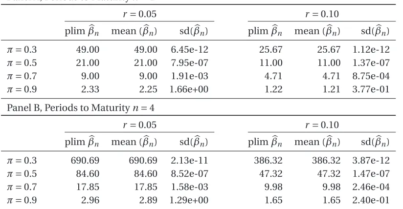
Table 1 shows how the theoretical value of the slope coefficient (plimβbn), computed
using expression (13), changes with values ofr ={0.05, 0.10},π={0.3, . . . , 0.9} andn=
{1, 4}. We observe that the size of the deviation of plimβbn from the EMH value of zero
depends crucially on the probability of the bubble regimeπ. This is to be expected since when a bubble develops but the probability of such an event occurring is small (e.g., π=0.3), there is a large difference between the realized future states of the economy (st+n) and the expectations of rational agents (ft,n). In these rare occasions, the deviation
of the slope coefficient from its EMH value is large. As the probability of the bubble regime increases, the difference between the future spot and the current forward rate narrows and the slope of the Fama regression approaches the EMH value.
–Table 1–
In many empirical applications, tests for bubbles are applied to small samples of data. A question that naturally arises is what are the small-sample properties of the least squares estimator (11) when the regression variables contain a bubble. To answer this question, we run a simulation experiment. In the experiment, we set the number of rep-etitions equal to 20,000, the sample size equal to 25,θ∼N(0, 1),ǫ∼N(0, 0.09) ,n∈{1, 4}, r ∈{0.05, 0.1}, andπ∈{0.3, . . . , 0.9}. The mean and standard deviation of the estimates are reported in Table 1 next to the theoretical values. Importantly, there is no evidence of bias with mean estimates being almost identical to theoretical values. Regarding the standard deviation, we observe that this statistic decreases withr and increases withπ, i.e., it decreases as the regression variables become more persistent, with very few ex-ceptions.
We have established that the slope coefficient in the Fama regression exceeds the EMH value when a bubble is ongoing and fundamentals follow a random walk. We note that this result cannot be generated by explosive fundamentals. Suppose that fundamen-tals follow an AR(1) process withφ>1 and there are no bubbles. The forward premium is given by
ft,n−st=(φn−1)νt, (14)
and
st+n−ft,n=ǫ′t+n, (15)
whereǫ′t+n=Pni=1φn−iθt+i. Substituting (14) and (15) into the expression for the least
squares slope coefficient yields
b β′n=
d
cov(ǫ′t+n,νt)
(φn−1)v ard(ν t)
.
The plim of the above expression is zero and, therefore, plimβb′n=βEMH. We conclude that, like unit root tests onst+n−ft,n, tests based onβbnallow the researcher to
Hypothesis Testing with a Persistent Regressor. Fama’s predictive regression (10) may contain a highly persistent, even explosive (under the alternative of bubbles), regressor which renders standard inference procedures invalid (see Campbell and Yogo, 2006; Ca-vanagh et al., 1995; Engsted and Nielsen, 2012; Jansson and Moreira, 2006; Phillips and Magdalinos, 2008). As shown by Stambaugh (1999), this inference problem may be fur-ther amplified if the innovations in Fama’s regression and the innovations of the forward premium are correlated, i.e. the regressor is endogenous.
Consider the following bivariate system
yt+1 = βxt+u1,t+1, (16)
xt+1 = ρxt+u2,t+1, (17)
whereyt+1=st+1−ft,1,xt =ft,1−st, and (u1,t+1,u2,t+1)′is a martingale difference
se-quence with finite fourth moment and possibly non-zero correlation coefficient δ= corr(u1,t+1,u2,t+1). Our objective is to test the null hypothesis of no bubbles or
equiva-lently no predictability (H0:β=0) against the alternative of an ongoing bubble (H1:β>
0) in the presence of uncertainty about the degree of regressor persistenceρ. It is typical in the predictive regression literature to model this uncertainty by adopting a local-to-unity setting whereρ=1+c/T. In this setting, widely employed test statistics, such as
t-ratios, have distributions that depend on the unknown localizing coefficientcand the correlation coefficientδ(see Cavanagh et al., 1995). Althoughδcan be consistently es-timated from the data, the nuisance parameterccannot, which leads to a nonstandard and nonpivotal inference problem.
Several methods have been proposed in the literature to bypass this problem. By far, the most popular are Bonferroni-type methods (Campbell and Yogo, 2006; Cavanagh et al., 1995; Hjalmarsson, 2011; Torous et al., 2004). These methods involve, first, inver-sion of a unit root test to construct confidence intervals forc (Stock, 1991), and, sec-ond, inversion of the nonpivotal limit distribution of the test statistic corresponding to the null hypothesis of no bubble, H0:β=0. Unfortunately, despite their popularity,
Bonferroni-type methods have some undesirable properties. In a recent paper, Phillips (2014) shows that confidence intervals constructed in the first stage of the testing pro-cedure are invalid at the limits of the domain of the localizing coefficient. The failure at the boundary has adverse implications for the performance of predictive regression tests. Specifically, for values ofρdistant from unity, thet-test of Cavanagh et al. (1995) is undersized, while the widely used two-sidedQ-test of Campbell and Yogo (2006) is over-sized, falsely rejecting the null of no predictability with probability approaching unity when in fact the null hypothesis is true.
stan-dard chi-square testing for a variety of autoregressive processes for the regressor, from stationary to mildly explosive, ii) it has good finite-sample properties (Kostakis et al., 2015), iii) it is straightforward to implement because it is based on linear regression, and iv) it can be extended to long-horizon predictive regressions (Phillips and Lee, 2013). For all these reasons, we adopt the IVX method and a rolling-window framework to test for bubbles (for a description of the IVX testing procedure see Appendix B).7
Forward and Futures Prices Although our theoretical analysis has focused on the for-eign exchange market, the proposed framework is general, and can be applied directly to any market for which forward or futures prices are available. It should be noted, how-ever, that in practice the distinct characteristics of forward and futures contracts may cause their prices to diverge, and thus lead to different estimation results. On the one hand, forward contracts are unstandardized, they trade over the counter, and they set-tle at maturity. On the other hand, futures contracts are standardized with respect to their size and maturity date, and they trade in organized exchanges, in which a clearing house guarantees against credit risk, and ensures that all profits and losses are settled at a daily basis (marking to market). As a consequence, futures contracts usually have lower default risk and are more liquid.8 Forward and futures contracts may also differ due to taxes, transaction costs, and margin requirements (Hull, 2015). Despite their dis-tinct characteristics, the findings of the empirical literature suggest that, for financial assets, the prices of these two types of derivative contracts are not significantly different and therefore, for our purposes, they can be treated as equivalent (see, Chow et al., 2000, and the references therein).
7Alternatives to Bonferroni-type methods are also provided by, among others, Jansson and Moreira
(2006) and Elliott et al. (2015). The first paper develops a conditional likelihood procedure based on a set of sufficient statistics. This testing procedure is theoretically appealing because it exhibits specific optimality properties in the local-to-unity model. However, simulation results in Kasparis et al. (2015) and Kostakis et al. (2015) show that, in practice, it exhibits substantial size distortions in cases of strong endogeneity. Moreover, Kasparis et al. (2015) find that there are severe difficulties with its numerical implementation. The second paper proposes a nearly optimal test that maximizes power over a range of values for the unknown
localizing parameterc. An attractive feature of this test is that it switches to a standardt-test when the
localizing coefficient estimate crosses a specific threshold and, thus, it avoids the problems of Bonferroni-type methods. Elliott et al. (2015) show that, for large sample sizes, the nearly optimal test displays good
properties and almost uniformly dominates theQ-test of Campbell and Yogo (2006). In our context, it is
im-perative that the testing procedure also displays good small-sample properties since periodically collapsing bubbles, if they exist, may be short-lived. However, the small-sample performance of the Elliott et al. (2015) test has not been explored yet. By conducting a battery of simulation experiments, we find that, for small samples, the Elliott et al. (2015) test exhibits severe oversizing when there is strong endogeneity, the regres-sor is stationary, and there is no prior knowledge of any nuisance parameters. On the other hand, the test is undersized in the presence of an explosive regressor - a property which may well be important when test-ing for speculative bubbles. The simulation results are available upon request. We are grateful to Michael Jansson for kindly providing his Matlab code, and to Graham Elliott for making his code available online http://econweb.ucsd.edu/~gelliott/RECENTPAPERS.htm.
8An exception is the foreign exchange market. Forward foreign exchange contracts are more actively
3 Monte Carlo Simulations
In this section, we examine the performance of the recursive unit root test and the rolling Fama regression in detecting and dating bubble episodes by conducting a battery of Monte Carlo experiments. The design of the experiments is similar to that of Phillips et al. (2015a) and allows us to investigate the role of a number of factors in the perfor-mance of the tests. These factors include the number of bubble episodes, the location of the bubble in the sample, the duration of the bubble, the probability of the bubble collapsing, the periods to maturity, and the bubble type.
3.1 Processes with a Single Bubble Episode
For our first Monte Carlo exercise, we consider a scenario with a single bubble episode which starts at timeτf =31, 51 or 71 and lasts ford=10, 15, or 20 periods. The sample
size in this and the following exercises is set equal toT =100 observations, the num-ber of repetitions is 1,000, the nominal significance level is 5 percent, and the values for the parameters describing the economy are, unless otherwise stated,π={0.5, 0.7},
r={0.05, 0.1},n=1,σǫ=0.3, andσθ=1.
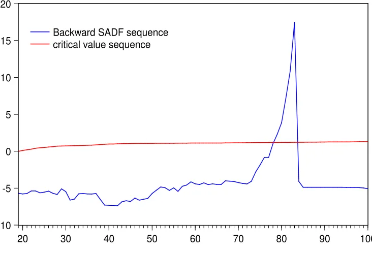
Before proceeding to the main Monte Carlo simulation results, we demonstrate the applicability of the two methods on one of the realizations generated with r =0.05, π=0.7,τf =71 andd=15. Figures 1 and 2 display test statistics (BSADF and IVX) and
95 percent critical value sequences for the Phillips et al. test and for the rolling Fama regression, respectively. Overall, the observed patterns are consistent with the theoret-ical analysis. Once the bubble starts the estimated test statistics gradually increase and eventually exceed their critical values rejecting the null hypothesis of no bubbles. When the bubble bursts both statistics fall below the critical bound almost instantaneously and remain there until the end of the sample.
–Figures 1 and 2–
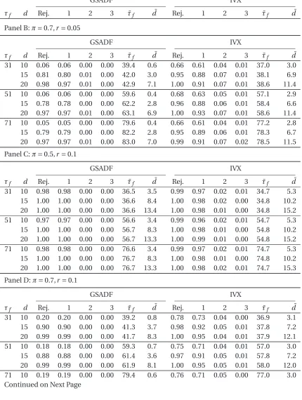
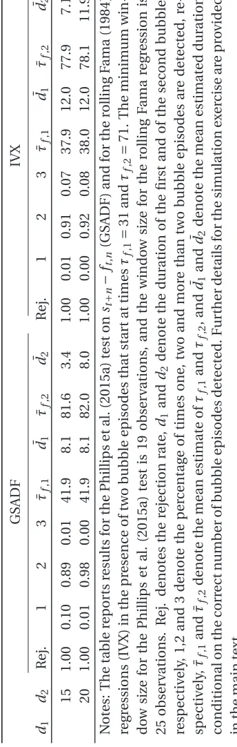
Regarding the main simulation results, Table 2 reports the empirical power of the tests Rej., the percentage of times one, two and more than two bubble episodes are de-tected, the mean estimate of the start date of the bubble ¯τf, and the mean estimated
duration ¯d. Several interesting conclusions emerge from the results. Starting with the empirical power, we observe that, for both tests, it increases with the duration of the bubbled and the structural parameterr, and it decreases with the probability of the economy being in the bubble regimeπ. The positive relation between empirical power and bubble duration is intuitively obvious and does not require explanation. As far as
r andπare concerned, these two factors determine the value of the AR coefficient in the bubble process (3) and, consequently, the degree of explosiveness ofst+n−ft,nand
the bubble process takes larger values, and the two variables that enter the Fama regres-sion equation become more explosive. This increase in the degree of explosiveness raises the power of the tests. Furthermore, it explains why, asπdecreases andr increases, the tests detect the bubble episode earlier (see ¯τf) and the mean estimated bubble duration
( ¯d) becomes longer.
–Table 2–
Turning to the comparison of the results for the two methods, we see that the em-pirical power of the rolling IVX test is similar to or higher than the recursive unit root test. The difference between tests is particularly apparent (about 60 percentage points) when the bubble durationdis short, the value forπis large, and the value forr is small. In other words, when the degree of explosiveness of the Fama variables is low, and the bubble is short-lived. A possible explanation for the superiority of the IVX over the unit root test in terms of power is that, under the null hypothesis of no bubble, thest+n−ft,n
process (9) is in fact stationary, rather than a unit root, which makes the unit root test conservative (see also the discussion of Phillips et al. (2015a, Section 5) about the appli-cation of unit root tests to price-to-fundamentals ratios).
With regards to date-stamping, the results in Table 2 (see ¯τf) suggest that the Fama
regression is again superior to the unit root test because it always detects earlier the emergence of the bubble. Both methods, however, perform remarkably well in detecting the collapse of the bubble, which is the reason the sum of ¯τf and ¯d is the same as the
date of collapse. The performance of the methods is also exceptional in terms of detect-ing the correct number of bubble episodes. Specifically, the maximum number of times that the methods falsely detect more than one bubble episodes never exceeds 6 percent of the total number of repetitions. Finally, it is worth noting that the location of the bub-ble does not affect the power of the tests, the time required to detect the bubbub-ble, ¯τf−τf,
and the mean estimated duration.
3.2 Processes with Two Bubble Episodes
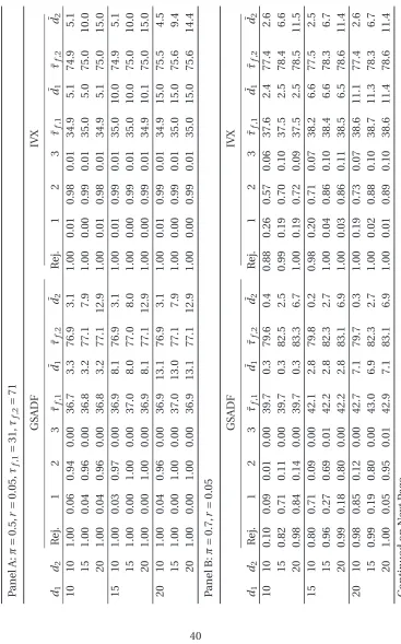
For the second Monte Carlo exercise, we consider a scenario with two bubble episodes, which start at times τf,1 =31 and τf,2 =71, and last for d1,d2 ={10, 15, 20} periods.
is not (i.e.,d1ord2equals 10 periods, andd16=d2),π=0.7, andr =0.05. For these
pa-rameter values, the Fama regression detects two bubbles in more than 70 percent of the cases, while the recursive unit root test in less than or equal to 14 percent of the cases. A possible reason for these large differences is that, as explained before, the recursive unit root test may be conservative, frequently failing to detect short-lived bubbles when the probability of being in the bubble regime is high, i.e. π=0.7. On the contrary, for π=0.5, both methods perform well in terms of power and detecting the correct number of bubble episodes.9
–Table 3–
3.3 Different Periods to Maturity,n
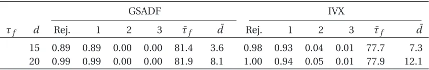
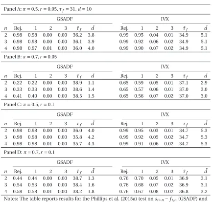
In the previous two simulation exercises, we set the number of periods to maturityn
equal to one. We now extend the analysis ton=2, 3 and 4. The simulation design is identical to that used for the one-bubble simulation exercise with the exception that we now consider a single starting dateτf =31, and a bubble duration ofd=10 periods.
–Table 4–
According to the results reported in Table 4, the number of periods to maturity has a substantial positive effect on the empirical power of the recursive unit root test for π=0.7 but has no effect forπ=0.5. Specifically, whennincreases from 2 to 4, the num-ber of rejections almost doubles (from 22 to 41 percent) forπ=0.7 andr =0.05, and it increases from 44 to 58 percent forπ=0.7 andr =0.1. Regarding the Fama regression, the empirical power of the IVX test does not appear to depend on the periods to maturity
n. However, it should be noted that asnincreases the Fama regression behaves slightly worse in detecting the correct number of bubble episodes. This property is not shared by the recursive unit root test. Overall, the conclusion that emerges from these results is that, as n increases, the performance of the Phillips et al. (2015a) test can improve substantially, which makes this test more attractive for largen.
3.4 Periodically Collapsing Bubbles
In the last simulation exercise, we examine bubble episodes that do not occur at a spe-cific part of the sample, as before, but instead emerge randomly. We also expand the
9We have run simulation experiments using DGPs with three bubble episodes. The results indicate that
analysis by considering the type of bubbles proposed by Evans (1991). This bubble DGP is given by
Bt+1= (
(1+r)Btηt+1, ifBt≤b,
h
λ+π1(1+r)ζt+1 ³
Bt−(1+1r)λ
´i
ηt+1, ifBt>b, (18)
whereλand b are positive constants with λ<(1+r)b, ηt+1 is a lognormal variable
scaled to have a mean of unity (that is,ηt+1=exp(κt+1−σκ2/2) whereκt+1∼N(0,σ2κ)), andζt+1 is a Bernoulli process that takes the value of one with probability πand the
value of zero with probability 1−π. Like Blanchard’s DGP, it is easy to verify that the DGP specified by (18) satisfies the condition for a rational bubble, i.e., Et[Bt+1]=(1+r)Bt.
However, contrary to Blanchard’s DGP, bubbles of the Evans’ type never fall to zero since
Bt >0 impliesBs>0 for alls>t. Consider, for example, a bubble that starts below the
thresholdb. The bubble initially grows at a constant expected rate of (1+r). Eventually the bubble exceedsb, and once this happens, its expected growth rate conditional on the bubble not collapsing increases to (1+r)/π. When the bubble collapses, it drops to a positive expected value ofλ, and the cycle begins again.
The fact that the expected growth rate conditional on the bubble erupting is greater than the unconditional expected growth rate implies a gap between the future spot and forward exchange rates. By adopting the framework of Section 2, it is straightforward to show that the difference between the two exchange rates is given by
st+n−ft,n = (1+r)n
à 1 π
n
Y
i=1
ηt+i−1
!
Bt+
µ 1−1
π ¶
λ
n
X
i=1 µ
1+r
π
¶n−i nY
j=i
ηt+j
+
n
X
i=1
φn−1θt+i. (19)
According to this expression, thest+n−ft,nprocess is explosive and does not depend on
fundamentals. Thus, the application of the recursive econometric tests is valid for the bubble DGP of Evans (1991).
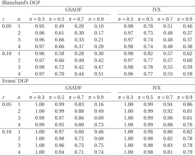
For the simulation exercise, we follow Evans (1991) and scale up bubbles gener-ated from (18) by a factor of twenty. Furthermore, we set the parameters of the two periodically collapsing bubble processes and of the process for fundamentals equal to π={0.3, 0.5, 0.7, 0.9},r ={0.05, 0.1},n={1, 2, 3, 4},λ=0.5,b =1,σǫ=0.3,σθ=1, and σκ=0.05. Finally, in order to make the analysis meaningful from a practical standpoint, we focus on bubble episodes that are not very short-lived, and discard series for which the duration of the longest bubble episode is less than or equal to five consecutive time periods. Table 5 presents the empirical power of the two econometric tests in this set-ting. Panel A reports results for the bubble DGP of Blanchard (1979), and Panel B for the bubble DGP of Evans (1991).
Overall, the results are in line with those for the previous simulation exercises. Both tests display very high power (equal to or greater than 95 percent) whenπis low. Asπ increases, their empirical power decreases. The decline becomes particularly apparent for the unit root test when the number of periods to maturitynand the structural pa-rameterr take small values. For instance, for the DGP of Evans withn=1 andr=0.05, the power of the GSADF drops from 100 to 16 percent asπincreases from 0.3 to 0.9, while the corresponding drop in power for the IVX test is from 100 to 86 percent.
The relationship betweenπand empirical power, however, is not always monotonic. Looking at the results forr=0.1 andπ={0.7, 0.9}, we observe cases where an increase in πis associated with higher (although slightly) empirical power. To explain this finding, we note that raisingπhas two opposite effects in the presence of periodically collaps-ing bubbles. On the one hand, similarly to the previous simulation experiments, when πincreases and the economy is in the bubble regime, the AR coefficient of the bubble process decreases, andst+n−ft,nandft,n−st become less explosive. As an implication,
an increase inπtends to lower the power of the tests. On the other hand, asπincreases, bubble episodes become more frequent, which tends to raise power. Hence, what our results suggest is that the overall effect is ambiguous and depends on the specific values of the DGP parameters.
Finally, a comparison of the results for the two tests (IVX and GSADF) reveals that the rolling Fama regression method is again more (in some cases substantially) powerful than the recursive unit root. In accordance with the findings from the previous simula-tion experiment, the difference between methods is large when the number of periods to maturitynis small and the probability of the bubble regimeπis high. Asnincreases the performance of the recursive unit root test generally improves, while the performance of the Fama regression remains the same or slightly worsens. As a consequence, forn=4, the difference in performance is substantially smaller -in some cases, less than 5 per-centage points.
4 Empirical Applications
In this section, we provide two empirical applications of the proposed bubble detec-tion methods to US dollar exchange rates. The first concerns the interwar German hy-perinflation, and the second the recent floating-rate period. We also illustrate how the proposed methods can be applied to stock market data, and, in particular, the S&P 500 index, using futures prices.
4.1 The German Hyperinflation
prob-lems. The starting date, on the other hand, corresponds to the change of convention to a four-week forward rate. The use of weekly data allows us to analyze a much larger sam-ple than those typically used in the German hyperinflation literature (see, e.g., Michael, Nobay, and Peel, 1994).
–Figures 3 and 4–
Figure 3 shows the evolution of the logarithm of the spot rate, st, over time. As it
is evident from the figure and well documented in the literature, the mark depreciated rapidly against the dollar in the early 1920s. At the start of our sample period, December 24th, 1921, a dollar was trading for 190 German marks. By August 11th, 1923, the same amount of dollars could buy more than three million marks, which implies an increase by a factor of 17 thousand in less than two years.
Similarly to other hyperinflations, the large movements in the exchange rate were mainly driven by the rate of money supply growth. A rapid monetary expansion started in the summer of 1921, when the German authorities adopted a policy of selling the mark to buy foreign currencies in order to pay World War I reparations, and finished in Novem-ber 1923 with the introduction of a new currency, the Rentenmark, which replaced the old currency at a conversion rate of one to a trillion. According to texts regarded as au-thoritative on the German hyperinflation (e.g., Bresciani-Turroni, 1937; Graham, 1930), the rate of growth of the money supply was the main but not the sole driving force of ex-change rate movements. A second factor that appears to have played an important role in the foreign exchange market at that time is destabilizing speculation. In his analysis of foreign exchange trading, Bresciani-Turroni (1937, p. 101) underlines the role of self-fulfilling beliefs in the determination of the exchange rate:“The dollar rate was increased rapidly from one day to the next and from one hour to the next by the expectation of a future rise”.The question we address in this section is whether speculative bubbles arose in the foreign exchange market.
–Table 6–
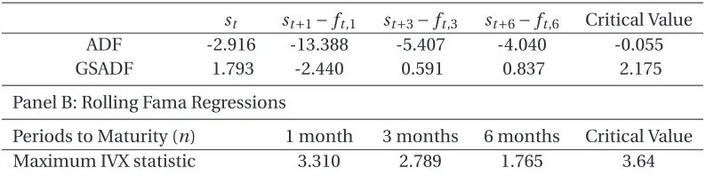
We begin our empirical analysis by examining the integration properties of spot and forward exchange rates. Perhaps surprisingly, despite a large amount of research on the German hyperinflation, the properties of these series have not been examined so far.10 The second and third columns of Table 6 report standard ADF and GSADF test statistics, respectively. The fifth column reports 95 percent critical values. The fact that the ADF statistics for the whole sample are greater than the 95 percent critical value indicates
10Funke et al. (1994) focus on Poland’s hyperinflation period and run a regime switching unit root test.
that the series have been explosive in the sample period. However, as shown in Section 2, explosive dynamics in asset prices does not constitute evidence neither in favor nor against bubbles since it may reflect bubbles or explosive market fundamentals, or both of these factors.
To shed light on the existence and duration of speculative bubbles, we investigate the integration properties of the difference between the future spot and forward rates,
st+4−ft,4, which is plotted in Figure 4. Looking at the results reported in the fourth
col-umn of Table 6, we observe that the GSADF statistic exceeds the 95 percent critical value but the ADF fails to do so. This implies that, although there are episodes of explosive dynamics, thest+4−ft,4series is not explosive throughout the sample period. The
con-clusion that emerges is that a speculative bubble process in the foreign exchange market exists, however, it is not ongoing for the entire sample -it collapses.
In order to identify the bubble period(s), we plot the BSADF statistics forst+4−ft,4
and the corresponding 95 percent critical value sequence in Figure 5.11 A comparison of the BSADF statistics with the critical value sequence suggests that self-fulfilling ex-pectations drove the German mark-US dollar away from market fundamentals in two occasions: in July-August 1922, and in July 1923. The bubble episodes are short-lived, with the second episode lasting a single period. Given the short duration of exuberance, it is not surprising that the GSADF test rejects the null of a unit root inst+4−ft,4, while
the standard ADF does not.
–Figures 5 and 6–
We complement the unit root analysis by running rolling Fama regressions. Figure 6 displays the sequence of IVX statistics together with 95 percent critical values. The maximum IVX statistic is 4.069, which is greater than the 95 percent critical value, and thus the null hypothesis of no bubbles is again rejected by the data. Overall, the observed pattern of the IVX statistic is very similar to that of the BSADF statistic. Starting below the critical value sequence at the beginning of the sample, the statistic rises and becomes significant in July 1922, indicating a first bubble episode. It then falls back below the critical value and remains insignificant until June 1923. In June 1923, the statistic starts increasing sharply again and exceeds the critical value sequence for the second time. This second bubble episode continues until August 1923 –a month before the authorities suspended forward trading in the German mark due to its rapid depreciation.
Interestingly, the two periods identified as consistent with speculative bubbles co-incide with those that Bresciani-Turroni (1937, p.102) gives as examples of destabilizing
11The minimum window size used for the recursive unit root test is 18 weeks, which is smaller than the
speculation that pushed the mark away from fundamental conditions: “For some time it was foreign speculation which provoked the great fluctuations of the exchanges...[ ] By August 1922 the dollar rate had risen beyond 1,900 marks; but a violent reaction set in and the dollar fell to little more than 1,200 marks...[ ] Towards the middle of August 1923 the dollar rate rose giddily to 1, 2, 3, and 5 million marks; later falling suddenly to 3 millions. These examples [] show that speculation did not exercise stabilizing influence on the ex-changes, but had rather the opposite effect.” Regarding the first period, Graham (1930, p.50) singles it out as representative of theflight from the mark: “The greatest effect ex-erted by speculators in exchange is ordinarily supposed to have occurred after the middle of 1922...”. Moreover, this period coincides with the peak deviation of the mark from its purchasing power parity. The gap between the internal value of the currency and its exchange value was the largest among all European countries at the time (for historical evidence on the misalignment of the currency see Graham, 1930, p.119).
Our analysis does not employ a specific model of exchange rate determination and, therefore, no direct conclusions can be drawn about the time series properties of market fundamentals. Nonetheless, the results of the standard ADF test onst and st+4−ft,4
taken together do provide indirect evidence. Bearing in mind thatst+4−ft,4 does not
depend on market fundamentals, whilest does, the fact that the standard ADF statistic
is insignificant for st+4−ft,4 but it is significant for st (see Table 6) suggests that the
process for market fundamentals is explosive. This conclusion is consistent with the finding of Flood and Garber (1980) of an explosive money supply process during the German hyperinflation. It also supports Nielsen’s (2008) view that hyperinflation data display explosive dynamics.
Before proceeding to the second empirical application, we would like to highlight two implications of the above results for standard statistical tests applied to the German hyperinflation. First, the fact that the process for market fundamentals is most likely explosive implies that statistical inference about bubbles based on unit root tests on spot prices alone is invalid. For this reason, either spot and forward rates should be used or an asset price determination model needs to be estimated. Second, because the identified bubble periods are short, standard statistical tests may fail to reject the null hypothesis of no bubbles, even if they are based on a correctly specified model, due to their low power. In this context, econometric models that allow for structural change, like the ones employed in this paper, seem more suitable.
4.2 The Recent Float
Thaler, 1990). During the period December 1980 to February 1985, the British pound price of the US dollar increased by more than 100 percent, from 0.418 to 0.924, which raised serious concerns about whether movements in the value of the dollar reflect only changes in macro fundamentals. Most notably, in June 1985, the then Federal Reserve Chairman, Paul Volcker, referred to anovervalueddollar and the possibility of a sharp decline (Feldstein, 1994). In line with Volcker’s statement, the results of several studies from that period suggest that it is very difficult to reconcile the large dollar appreciation with the predictions of conventional economic models (based on variables such as in-flation rates, interest rate differentials, and relative income) and thus other factors must also be taken into account, such as speculative bubbles (see, for instance, Evans, 1986; Sarno and Taylor, 2002).
In this section, we re-examine the presence of speculative bubbles in the British pound-US dollar foreign exchange market by applying the two methods proposed in Sec-tion 2 to monthly data on spot and forward rates for the period January 1979 to Decem-ber 2013. The data is downloaded from the Bank of England websitehttp://www.
bankofengland.co.uk/. An advantage of using data for the recent float, in
com-parison to data for the interwar period, is the greater availability of forward rates, which allows us to obtain and compare results for different periods to maturity; namely one, three, and six months.
–Figures 7 and 8–
Figures 7 and 8 show the evolution of the logarithm of the spot rate and the difference between the logarithm of the future spot and the logarithm of the six-month forward over time. It is evident from Figure 7 that the long swings in the British Pound-US dollar rate is not a phenomenon unique to the 1980s. For instance, in the first half of 2000s, the dollar experienced another long (but not as extreme as that of the 1980s) period of depreciation, with the spot rate falling by more than one-third from June 2001 to October 2007, and then rebounding a year later. Thus, different periods of exuberance in the foreign exchange market may exist during the recent float. Turning to the time series plot of the difference between future spot and forward rates (Figure 8), we observe large and persistent deviations from the EMH value of zero, especially in the 1980s, early 1990s, and mid-to-late 2000s. However, the series does not exhibit trend-like behavior over very long time periods like the spot rate, which suggests a lower degree of persistence.
–Table 7–
column) and, although this gap narrows as the number of periods to maturity increases, it remains substantial.12 What is more important is that, according to the results, the null hypothesis of a unit root cannot be rejected in favor of the alternative of explosive dynamics at the 5 percent significance level for any of the series examined. The fact that the unit root tests cannot detect any period of exponential growth, even in the spot rate, suggests that there is no evidence in favor of rational speculative bubbles. This is also the conclusion that emerges from the results for rolling Fama regressions. Looking at Panel B of Table 7, we observe that, irrespective of the number of periods to maturity, the maximum IVX test statistic is below the 95 percent critical value. As an implication, the slope of the Fama regression never significantly exceeds the EMH value and, therefore, the no-bubbles hypothesis cannot be rejected.
In contrast to our findings, the studies of Meese (1986) and Evans (1986) provide evidence in support of speculative bubbles in the British pound-US dollar rate in the early 1980s. A possible explanation for the discrepancy between the former study and ours is related to the joint hypothesis problem. In particular, Meese (1986) employs the Hausman-type test of West (1987) which relies on a particular economic model and, con-sequently, may falsely reject the null hypothesis due to an erroneous assumption about fundamentals.13 Regarding the latter study, Evans (1986) advocates a test that exploits the fact that the median of excess returns is different from zero in the presence of pe-riodically collapsing bubbles. However, as Evans (1986) points out, a nonzero median may arise due to factors other than bubbles, such as nonsymmetric innovations of fun-damentals. That is, the test is based on a necessary but not a sufficient condition for bubbles.
4.3 The US Equity Market
As a final application, we examine the US equity market. Our monthly dataset includes the S&P 500 price index, an observed market fundamental series (namely, S&P 500 div-idends), and S&P 500 futures prices for horizons of three, six, and nine months.14 The first two series are downloaded from Robert Shiller’s website and the remaining from Bloomberg. The dataset starts in December 1982, which corresponds to the commence-ment of S&P 500 futures trading on the Chicago Mercantile Exchange in April of the same year, and ends in March 2015.
–Figures 9 & 10–
12Unit root tests results for one-, three-, and six-month forwards rates are not reported because they are
virtually identical to those for the spot rate.
13Meese (1986, p. 367) too recognizes the possibility that the economic model adopted may not be
well-suited for the dollar-pound rate.
14We follow Chernenko et al. (2004) and obtain regularly-spaced futures prices by linearly interpolating
Figure 9 displays the logarithm of the real S&P 500 price index. As can be seen from the figure, the period under examination is characterized by a number of market rallies followed by market crashes (for a historical perspective, see Mishkin and White, 2002, and Shiller, 2015). The most remarkable episode is the great surge of the 1990s, the so-calledmillennium boom. In April 1994, the S&P 500 index stood (in nominal terms) at 447 units. In the subsequent years, stock prices increased at an unprecedented rate, which led Alan Greenspan to talk aboutirrational exuberancein the stock market, and by the early 2000s the index had more than tripled, to 1485 units. This rapid price in-crease was followed by a dramatic market crash. During the crash, the S&P 500 index lost in a few years almost 44 percent of its value, reaching a minimum of 837 units in February 2003. With the exception of the famous stock market run-up and collapse of the 1920s, no other historical episode comes close to resembling the behavior of the S&P 500 around 2000. Two other stock market episodes that, although lesser than the mil-lennium boom, are worth noting are:Black Mondayin October 1987 when, following a surge of stock prices, the S&P 500 index fell by about 20 percent, setting a new record one-day decline (see Carlson, 2006); and the 2007-2009 US bear market, during which the S&P 500 index lost around 50 percent of its value. As illustrated in Figure 10, which depicts the S&P 500 price-to-dividend ratio, and as argued by Shiller (2015) and many other authors, it is difficult to reconcile these stock price movements with the behavior of observed market fundamentals.
–Table 8–
To investigate the existence of speculative bubbles in the US stock market, we run unit root tests on the logarithm of the real S&P 500 price index, s∗t, the logarithm of the price-to-dividend ratio,st−dt, and the difference between the logarithm of the
fu-ture spot price and the logarithm of the fufu-tures price, st+n−ft,n withn=3, 6, and 9
months. We also run rolling Fama regressions. All results are reported in Table 8. By focusing on the GSADF test statistics (Panel A), we observe that the null hypothesis of non-explosive behavior can be rejected at the five percent significance level for all series but one, st+3−ft,3. The finding that the S&P 500 price index and the S&P 500
price-to-dividend ratio display episodes of explosive dynamics is in accordance with the re-cent empirical literature on bubbles in the US stock market (see, e.g., Homm and Bre-itung, 2012; Phillips et al., 2015a). Our study complements this literature by showing thatst+6−ft,6 andst+9−ft,9also display explosive dynamics. By doing so, it provides
power of the IVX test declines with the maturity horizon (see Section 3) which may ex-plain why the test fails to reject the null of no-bubbles for maturity horizons of six and nine months, while the GSADF does so.
–Figures 11, 12 & 13–
For identifying the periods of exuberance, we plot the sequence of BSADF statistics together with the corresponding 95 percent critical value sequence for the logarithm of the real S&P 500 price index,s∗t, the logarithm of the S&P 500 price-to-dividend ratio,st−
dt, and the difference between the logarithm of the future spot index and the logarithm
of the futures price index,st+9−ft,9, in Figures 11, 12, and 13, respectively. As can been
seen from the two former figures, the BSADF test detects three episodes of exuberance in the real S&P 500 index and in the price-to-dividend ratio. These three episodes are also identified in the study of Phillips et al. (2015a), and correspond closely to Black Monday in October 1987, the millennium boom, and the US bear market of 2007-09. Turning tost+9−ft,9, we observe that the BSADF test detects the latter two episodes but fails to
detect speculative dynamics for Black Monday. By comparing the results fors∗t andst−dt
with those forst+9−ft,9, we also observe that the period of exuberance corresponding
to the millennium boom is shorter and takes place slightly later in the sample for the
st+9−ft,9series.
In summary, the above analysis suggests that episodes of exuberance do exist in the US stock market. This conclusion holds when controlling for observed market funda-mentals, and when futures prices are used to avoid specifying the asset pricing model, with the latter approach yielding somewhat more conservative results.
5 Conclusions
model of asset price determination, are robust to an explosive root in the process for fundamentals, and are accompanied by date-stamping strategies.