warwick.ac.uk/lib-publications
Manuscript version: Author’s Accepted Manuscript
The version presented in WRAP is the author’s accepted manuscript and may differ from the
published version or Version of Record.
Persistent WRAP URL:
http://wrap.warwick.ac.uk/113233
How to cite:
Please refer to published version for the most recent bibliographic citation information.
If a published version is known of, the repository item page linked to above, will contain
details on accessing it.
Copyright and reuse:
The Warwick Research Archive Portal (WRAP) makes this work by researchers of the
University of Warwick available open access under the following conditions.
Copyright © and all moral rights to the version of the paper presented here belong to the
individual author(s) and/or other copyright owners. To the extent reasonable and
practicable the material made available in WRAP has been checked for eligibility before
being made available.
Copies of full items can be used for personal research or study, educational, or not-for-profit
purposes without prior permission or charge. Provided that the authors, title and full
bibliographic details are credited, a hyperlink and/or URL is given for the original metadata
page and the content is not changed in any way.
Publisher’s statement:
Please refer to the repository item page, publisher’s statement section, for further
information.
Cost-Benefit Analysis of Moving-Target Defense in
Power Grids
Subhash Lakshminarayana
∗and David K.Y. Yau
∗†∗ Advanced Digital Sciences Center, Illinois at Singapore, Singapore 138602
† Singapore University of Technology and Design, Singapore 487372
Email: ∗subhash.l@adsc-create.edu.sg,† david yau@sutd.edu.sg
Abstract—We study moving-target defense (MTD) that
ac-tively perturbs transmission line reactances to thwart stealthy false data injection (FDI) attacks against state estimation in a power grid. Prior work on this topic has proposed MTD based on randomly selected reactance perturbations, but these perturbations cannot guarantee effective attack detection. To address the issue, we present formal design criteria to select MTD reactance perturbations that are truly effective. However, based on a key optimal power flow (OPF) formulation, we find that the effective MTD may incur a non-trivial operational cost that has not hitherto received attention. Accordingly, we characterize important tradeoffs between the MTD’s detection capability and its associated required cost. Extensive simulations, using the MATPOWER simulator and benchmark IEEE bus systems, verify and illustrate the proposed design approach that for the first time addresses both key aspects of cost and effectiveness of the MTD.
I. INTRODUCTION
Cyber attacks against critical infrastructures can lead to severe disruptions. The December 2015 attack against the Ukraine’s power grid was a real-world example, which caused power outages for a large number of customers for hours [1]. These attacks were typically crafted by sophisticated attackers, sometimes with national backing, who managed to spend considerable time inside a system to learn its operational details, and accordingly designed the injection of malicious data/control to disrupt its operations [2]. It is thus imperative to design counteracting defense approaches to defeat the knowledgeable attackers. Moving-target defense (MTD) [3] is a defense approach that has received increasing attention. It is based on dynamically changing the system parameters that attackers need to target for customizing their attacks, in order to invalidate the attackers’ prior knowledge of the system and render ineffective any of their prior designed strategies. It has the potential to make it extremely difficult or impossible for would-be attackers to keep up with the system dynamics.
In this paper, we focus onfalse data injection(FDI) attacks against state estimation (SE) in power grids. SE is a key method for grid operators to obtain a best estimate of the system state from noisy sensor measurements collected via a supervisory control and data acquisition (SCADA) system,
This work was supported by the National Research Foundation (NRF), Prime Minister’s Office, Singapore, under its National Cybersecurity R&D Programme (Award No. NRF2014NCR-NCR001-31) and administered by the National Cybersecurity R&D Directorate.
for example. Its output is used in critical applications such as economic dispatch (for profits) and contingency analysis (for reliability). A bad data detector (BDD) associated with the SE is often deployed for identifying bad data (e.g., sensor anomalies and FDI attacks) to ensure trustworthy results. However, it has been shown [4] that FDI attacks crafted using detailed knowledge of a power grid’s topology and the reactance settings of its transmission lines can bypass the BDD and remain stealthy. Such an undetected attack can have severe consequences, e.g., trips of transmission line breakers or unsafe frequency excursions [5], [6].
To strengthen the BDD, it has been shown that if a carefully chosen subset of the sensors can be well protected (e.g., by tamper-proof and encryption-enabled PLCs), or if a key subset of the state variables can be independently and reliably verified by phasor measurement units (PMUs) deployed at strategically chosen locations, then a BDD-bypassing FDI attack becomes impossible [7], [8], [9]. However, a major revamp of the basic sensing infrastructure can be quite expensive (e.g., PMU has high cost [10]) or infeasible for the many existing legacy systems whose life cycles often last decades and which are not expected to retire for the foreseeable future. Alternatively, FDI attacks can be significantly mitigated by MTD that invalidates the knowledge attackers used for crafting their prior attacks, specifically by active perturbation of the grid’s transmission line reactance settings in our application context [11], [12], [13]. This approach is practical because of current D-FACTS devices capable of active impedance injection [14]. Because of their low cost and ease and flexibility of deployment, they are being increasingly installed in existing alternating-current (ac) transmission networks to control power flows [15].
characterization of effective MTD, prior work has not been able to address explicitly the associated cost involved. Rather, it is assumed that the MTD can be always constrained to have negligible or some “low enough” operational cost [13], [11]. However, MTD designed with any absolute cost constraints will not be useful if the MTD does not perform. It is thus critical to understand the inherent cost-benefit tradeoff of the MTD to accordingly inform system operators (SOs) in their choice of security policies, which is a key objective of this paper.
To achieve our goal, we analyze the problem of selecting MTD reactance perturbations that jointly consider their effec-tiveness (i.e., capability of attack detection) and operational cost (i.e., economic inefficiency). As in prior work, we assume that the attacker has learned the system configuration initially and uses this knowledge to craft stealthy FDI attack vectors, but the attacker cannot track the reactance perturbations with-out significant delays. In this setting, large MTD perturbations will cause the actual system to deviate significantly from the attacker’s prior knowledge, so that a large majority of the previously stealthy FDI attacks will now likely become detectable. Conversely, however, the large perturbations will also cause the power grid to operate significantly away from the optimal state, thereby incurring a significantly higher economic cost. On the other hand, smaller perturbations will be less expensive, but risk more undetected attacks. The general cost-benefit tradeoff is thus interesting.
In this paper, we address the cost-benefit tradeoff of the MTD by formulating its perturbation selection as a constrained optimization problem, namely minimization of the operational cost subject to a given effectiveness constraint. The opera-tional cost is quantified as the increment due to the MTD over the cost achieved at optimal power flow (OPF) of the system without MTD. This cost is always non-negative. The effectiveness is quantified as the fraction of prior stealthy FDI attacks (i.e., those before the MTD perturbation) that will become detectable by the BDD after the perturbation. It is difficult to give an exact analysis of the effectiveness. We will instead employ a heuristic metric that effectively invalidates the attacker’s knowledge required to bypass the BDD. Extensive simulation results show that the heuristic metric effectively approximates the true metric.
We use a direct-current (dc) power flow model to approx-imate power flows in an alternating-current (ac) grid. This approach is widely adopted and well justified in power system research (e.g., [4], [7], [13]). Under the dc model, the OPF cost corresponds mainly to the cost of generation dispatch. Moreover, the sensor measurements are linearly related to the system state through a measurement matrix, which in turn depends on the power grid topology and the reactance of the transmission lines. Naturally, perturbing a branch reactance will alter the measurement matrix correspondingly. A key observation in our analysis is that the MTD’s effectiveness and operational cost are related to the separation between the column spaces of the measurement matrices before and after the MTD. While the effectiveness is enhanced by increasing
the separation between the two column spaces, the operational cost increases. Therefore, different degrees of separation be-tween the two spaces provide a spectrum of balance bebe-tween the two metrics.
We note that, in light of our deliberate cost analysis of the MTD, the MTD can be viewed as a form of insurance against possible FDI attacks. Such insurance requires an ongoing payment of “premiums” irrespective of whether an attack occurs or not. However, in the event of an attack, which may be accumulatively extremely expensive if allowed to persist indefinitely because of lack of detection, the insurance can provide a much needed hedge against the damage. In actual deployments, whether to procure such insurance (i.e., turn on the MTD or not) is likely a matter of diverse factors such as institutional policies (including the institution’s attitude towards risk taking), estimated vulnerability to attacks or likelihood of attacks, and the cost-benefit tradeoff specific to the power grid in question. This paper sheds light on tradeoffs in the key technical problem, which serves as an important reference basis for the other questions. Nevertheless, it does not attempt to answer all the questions, particularly policy questions, that are also interesting.
The main contributions of the paper are summarized as follows:
• We derive conditions for an MTD reactance perturbation to ensure that no FDI attacks crafted based on the out-dated (pre-perturbation) system configuration will remain stealthy after the perturbation.
• When the reactance adjustment capability of D-FACTS is
insufficient for achieving the above condition, we present heuristic design criteria for selecting MTD perturbations that can still highly likely achieve effective attack detec-tion.
• We characterize the tradeoff between the MTD’s effec-tiveness and its operational cost in a constrained opti-mization framework. Additionally, we present extensive simulation results using the realistic MATPOWER sim-ulator for benchmark IEEE bus systems to verify and illustrate the tradeoff.
The remainder of this paper is organized as follows. Sec-tion II reviews related work. SecSec-tion III introduces the pre-liminaries. Section IV explains the attacker and the defender model. Sections V and VI analyze the MTD’s effectiveness and its cost-benefit tradeoff. Section VII presents simulation results. Section VIII concludes. The technical proofs can be found in Appendices A,B and C.
II. PRIORWORK
can also be crafted using the eavesdropped measurement data only. The impact of such stealthy FDI attacks on system efficiency and safety were investigated. In particular, the economic impact of FDI attacks were studied in [19] and [20]. Reference [6] showed that the attacker can drive the power system frequency to unsafe levels by injecting a sequence of carefully-crafted FDI attacks.
To address BDD’s vulnerability, defense mechanisms based on protecting a strategically-selected set of sensors and their data links were proposed [7], [8], [9]. The use of generalized likelihood ratio test was proposed to detect FDI attacks when the adversary has access to only a few meters in [21]. Reference [22] presented a sparse optimization based approach to separate nominal power grid states and anomalies.
The concept of MTD was originally proposed for enterprise networks based on changing the IT features of devices such as end hosts’ IP addresses and port numbers, the routing paths between nodes, etc. [23], [24]. More recent work has proposed MTD in power systems by changing its physical characteristics [11], [12], [13]. In particular, on-going FDI attacks can be detected by introducing reactance perturbations that are known only to the defender (SO) [11], since the change in sensor measurements (after the perturbations) will be different from its predicted value based on the power flow model (due to the attack). It has also been shown that stealthy FDI attacks can be precluded by actively perturbing the branch reactances to invalidate the attacker’s knowledge [13]. We similarly consider MTD for power systems in this paper. Compared with the prior work, ours is the first to jointly consider the MTD’s effectiveness and its operational cost. We provide hitherto unavailable formal design criteria for selecting effective MTD reactance perturbations, and expose important tradeoffs between the effectiveness and operational cost.
III. PRELIMINARIES
Power Grid Model
We consider a power network that is characterized by a set
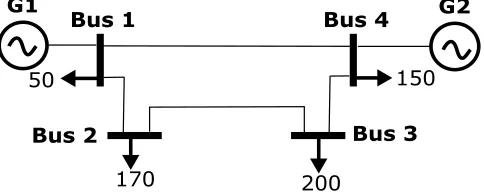
N = {1, . . . , N} of buses, L = {1, . . . , L} of transmission lines (an example of the 4 bus power system is shown in Figure 3). The line l ∈ L that connects bus i and bus j is denoted by l = {i, j}. The time of operation is denoted by
t∈
R
.At busi, we denote the power generation and load at time
t byGi,t andLi,t respectively and the reactance of linkl by
xl,t.We adopt the dc power flow model [25], under which the
power flow on line l at timetdenoted by Fl,t, is given by
Fl,t= 1
xl,t
(θi,t−θj,t),
whereθi,t andθj,tare the voltage phase angles at busesi, j∈ N respectively at timet. For safe operation, the branch flows must be maintained within the power flow limits Fmax
k at all
time, i.e.,
−Fkmax≤Fk,t≤Fkmax, ∀t.
The relationship between branch power flows and the voltage phase angles can be compactly represented asft=DtATθt,
where the matrix A ∈
R
N×L is the branch-bus incidence matrix given byAi,j=
1, if linkj starts at busi,
−1, if linkj ends at busi ,
0 otherwise,
andDt∈
R
L×L is a diagonal matrix of the reciprocal of linkreactances, i.e.,
Dt=diag
1
x1,t
, 1 x2,t
, . . . , 1 xL,t
,
and ft = [F1,t, . . . , FL,t]T (similarly gt,lt,θt denote the
vector forms of the corresponding quantities).
We assume that a subset of the linksLD⊆ Lare equipped with D-FACTS devices, and the reactances of these links can be changed within the range [xmin,xmax], wherexmin,xmax are the reactance limits achievable by the D-FACTS devices. Naturally, xminl =xmaxl =xl,t if l /∈ LD. Denote the vector
of branch reactances byxt.
State Estimation & Bad Data Detection Technique
SE is a technique of estimating the system state from its noisy sensor measurements [25]. Under the dc power flow model, the state at time t corresponds to the nodal voltage phase angles θt, which are monitored by a set of
M measurements zt ∈
R
M. The measurements correspondto the nodal power injections, and the forward and reverse branch power flows, i.e.zt= [˜pt,˜ft,−˜ft]T.We note that the
measurements may be different from the actual values of pt
andftdue to sensor measurement noises or cyber-attacks. The
measurement vector and the state are related as
zt=Htθt+nt,
where nt is the measurement noise, which is assumed to
have Gaussian distribution. Ht∈
R
M×Nis the measurement matrix given by
H=
DtAT −DtAT ADtAT
.
The estimate of the system state, θbt, is computed using a
maximum likelihood (ML) estimation technique, given by [25],
b
θt= (HTtWHt)−1HTtWzt,
whereWis a diagonal weighting matrix whose elements are reciprocals of the variances of the sensor measurement noise. A BDD is used to detect faulty sensor measurements. It compares the residual defined by rt = ||zt−Htθbt|| against a pre-defined thresholdτ and raises an alarm ifrt≥τ.The
Fig. 1: System block diagram.
Undetectable FDI Attacks
We consider FDI attacks against the SE, in which the attacker injects an attack vector at ∈
R
M into the sensormeasurements, i.e.,zat =zt+at,wherezat is the measurement
vector under an attack. In general, the BDD can detect arbitrary FDI attack vectors. However, it is demonstrated [4] that the BDD’s detection probability for attacks of the form at=Htc, wherec∈
R
N
, is no greater than the FP rate α. Such attacks are referred to as undetectable attacks.
Optimal Power Flow Problem
OPF is an optimization framework to adjust the power flows in the network (by setting the generator dispatch and the branch reactances) with the objective of minimizing the generation cost for a given load vector lt ∈
R
N, stated asfollows1:
COPF,t= min
gt,xt
X
i∈N
Ci(Gi,t) (1a)
s.t. gt−lt=Btθt, (1b) −fmax≤ft≤fmax, (1c) gmin≤gt≤gmax, (1d) xmin≤xt≤xmax, (1e)
where Ci(Gi,t)is the cost of generating Gi,t units of power
at node i ∈ N, the matrix Bt = ADtAT. In (1), the first
constraint (1b) represents the nodal power balance constraint, i.e., the power injected into a node must be equal to the power flowing out of the node. Constraints (1c)-(1e) correspond to the branch power flows, generator limits, and D-FACTS limits, respectively. We denote gt∗,x∗t = arg maxgt,xtOPF. We note that the OPF cost depends on the branch reactances through the matrixBt (in addition to the loads).
IV. MOVING-TARGETDEFENSE INPOWERGRIDS
A. Attacker and the Defender Model
A block diagram of the system under study is shown in Fig. 1. We consider a strong attacker who has access to the measurement data communicated between the field devices and the control center. Such access could be obtained by exploiting vulnerabilities in power grid communication
1In the absence of D-FACTS devices installed within the grid, OPF
optimizes over the generator dispatch values only (which is the version of OPF traditionally used [25]).
Pre-perturbation Post-perturbation
Time between MTD
Ht H0t0 Measurement
Matrix
Time
Time between MTD
t t0
[image:5.612.58.285.58.147.2]Time
Fig. 2: MTD timeline. The vertical arrows indicate the times at which the system is perturbed.
systems. For example, in modern-day power grids, the field devices (such as remote terminal units) are often IP-accessible [26]. We also assume that the attacker can learn the system’s measurement matrix (using the eavesdropped measurements) and craft undetectable FDI attacks accordingly (e.g., see [17], [18]).
Under MTD, the defender (e.g., the SO) tries to thwart the FDI attacks by actively perturbing the transmission line reactances to invalidate the attacker’s prior knowledge. We assume that at the time of introducing MTD perturbations, there are no on-going FDI attacks. Note that the power system under consideration is naturally dynamic (even without MTD) since the branch reactances are optimized periodically to reflect temporal changes in the system load (refer to the OPF problem in (1)). However, these natural changes are usually insufficient for effectively negating the attacker’s knowledge. Thus, the defender deliberately introduces an additional reac-tance perturbation to ensure the MTD’s detection capability.
The defender implements the MTD reactance perturbations by sending MTD control commands to the remote D-FACTS devices in the grid. Unlike the sensor measurements that support the grid’s normal operation (e.g., extensive SCADA measurements collected every few seconds), these commands are much less frequent (e.g., hourly, see the discussion below), have much more restricted scope (i.e., between the control center and the set of D-FACTS devices only), and do not have stringent real-time constraints. Hence, we assume that it is feasible to encrypt the MTD commands to ensure their confidentiality.
We note that although the attacker cannot read the MTD commands directly due to their encryption, in principle he may still infer the MTD perturbations by monitoring their effects on the eavesdropped sensor measurements and estimating the new measurement matrix accordingly. Thus, the secrecy of the MTD generally decays over time. In practice, however, the learning will be time consuming since the attacker must collect an informative sequence of the measurements over a significant duration of time. In this paper, we assume that the time interval between the MTD perturbations is sufficiently small, so that during it the attacker’s gain in knowledge (of the measurement matrix) is negligible.
G1
Bus 4 Bus 1
170
G2
Bus 2 Bus 3
200
[image:6.612.321.558.44.159.2]150 50
Fig. 3: 4 bus system under consideration. The loads are indicated in MWs.
maximum information diversity in that they are i.i.d. Hence, if we assume optimistically for the attacker that SCADA measurements need to be only5−10seconds apart to achieve the information diversity, their result suggests that the time required by the attacker to learn the system sufficiently well for stealthy attacks is on the order of a few hours. Accordingly, hourly MTD perturbations might be realistic for practical systems. Further, we note that utilities typically solve the OPF more frequently, i.e., every 5−10minutes (whereas we only need to update the MTD every hour or so). Thus, between the MTD updates, the OPF will be solved as in (1).
The MTD timeline is illustrated in Fig. 2. We consider two representative time instants t andt0 at which the reactances are perturbed for MTD. We denote the branch reactances and the measurement matrix after applying the MTD perturbations by x0t0 = [x01,t0, . . . , x0L,t0]T and H0t0 respectively, and the
reactance perturbation vector by ∆xt,t0 =xt−x0t0. We note
that in the absence of MTD, the branch reactances and the measurement matrix would be set to xt0 andHt0 by solving
(1) at time t0.
In the rest of the paper, we address the question of how to select MTD perturbations that are effective in detecting FDI attacks crafted based on the outdated (i.e., pre-pertubation) knowledge, and examine their cost-benefit tradeoff. We use
a0t0 to denote the value of a power system parameterat after
the MTD. E.g., θ0t0 denotes the nodal voltage phase angles
after the MTD. To motivate our inquisition, we now illustrate an example to show that certain randomly selected MTD perturbations will remain vulnerable to FDI attacks crafted with the attacker’s pre-pertubation knowledge of the system.
B. A Motivating Example
We consider the 4-bus example shown in Fig. 3 [27]. For simplicity, we assume that the system load is fixed (indicated in Fig. 3) and does not change with time. Furthermore, the pre-perturbation system state and the reactance settings xt (and Ht) are adjusted by solving (1). The resulting branch flows,
generation values and OPF cost are listed in Table II. The attacker is assumed to have learned the pre-perturbation matrix Ht.
To implement the MTD, we consider four reactance perturbation vectors respectively given by ∆x(1)t,t0 = η[x1,0,0,0]T, ∆x
(2)
t,t0 = η[0, x2,0,0]T,∆x (3)
t,t0 =
r0(1) r0(2) r0(3) r0(4)
Attack1 2.82 2.87 0 0
Attack2 0 0 2.87 2.82
TABLE I: BDD residual values.
Line Flow (MWs) Gen. (MWs) Cost($)
Line 1 Line 2 Line 3 Line 4 Gen 1 Gen 2
[image:6.612.55.297.52.149.2]1.15× 10⁴ 126.56 173.44 -43.44 -26.56 350 150
TABLE II: Pre-perturbation power flows, generator dispatch and OPF cost for 4-bus system.
MTD Gen. (MWs) OPF Cost ($)
∆x1 337.37 162.62 1.1626×10⁴
∆x2 340.51 159.48 1.595×10⁴
∆x3 348.62 151.37 1.1514×10⁴
∆x4 345.95 154.02 1.154×10⁴
TABLE III: Post-perturbation generator dispatch and OPF cost.
η[0,0, x3,0]T, ∆x (4)
t,t0 = η[0,0,0, x4]T, where η is the percentage change in the reactance relative to its initial value. We assess each of the four MTD perturbations in terms of (i) attack detection and (ii) operational cost.
For attack detection, we inject an attack of the form a = Htc into the modified power network (after the MTD), and
examine its BDD residual. For illustration, we consider two attacks – attack 1 in which c = [0,1,1,1]T and attack 2 in
which c = [0,0,0,1]T – and set η = 0.2. For simplicity,
we ignore measurement noises. The BDD residuals under the four MTD perturbations are listed in Table I. Note that in the absence of measurement noise, a non-zero value of the residual indicates the presence of attack. We observe that for each of the four perturbations, there exist attack vectors of the form a = Htc, which continue to bypass the BDD for the
perturbed power network.
We also enlist the post-pertubration OPF cost in Table III. We observe that the OPF cost increases in each of the four cases, compared to its pre-perturbation cost, and the perturbation∆x3 incurs the least cost.
C. MTD Perturbation Selection Challenges
Based on the above illustrating example, we make the following conclusions. First, it is evident that a subset of the attacks of the form a = Htc continue to bypass the
[image:6.612.354.517.196.266.2]sections, we characterize formally the MTD’s effectiveness and its operational cost, and present a framework for choosing appropriate MTD perturbations that balance between the two concerns.
V. MTD’SEFFECTIVENESS OFATTACKDETECTION
In this section, we address the problem of selecting effective MTD reactance perturbations from an attack detection point of view. The goal is to select reactance perturbations within the physical constraints of the D-FACTS devices to effectively invalidate the attacker’s knowledge for bypassing the BDD. The section is divided into two parts. In the first part, we devise a metric to quantify the effectiveness of the MTD. In the second part, we derive the conditions and propose design criteria for MTD perturbations to preclude stealthy FDI attacks in practice.
Henceforth, we use the notation “MTD H0t0” to refer to a
reactance perturbation that changes the measurement matrix fromHttoH0t0.We letAdenote the set of all attack vectors
of the form a=Htc,i.e.,
A={a:a=Htc,||a|| ≤amax,c∈
R
N}.For an attack vector a, we let P0
D(a) denote its detection
probability under MTD H0t0, where PD0 (a) = P(r0 ≥ τ).
We denote by A0(δ) ⊆ A the subset of attacks in A whose
detection probability under MTD H0t0 is greater than a given
δ∈[0,1],i.e.,
A0(δ) ={a:a=H
tc,||a|| ≤amax, PD0(a)> δ,c∈
R
N}.
A. Metric to Quantify MTD’s Effectiveness
First, we devise a metric to quantify the MTD’s effective-ness. Intuitively, an MTD perturbation “A” is more effective than a perturbation “B” if it can detect more FDI attacks in the set Awith high probability. However, A, a subset in the
n-dimensional space (
R
n), has infinitely many attack vectors. For these sets, theLebesgue measuregeneralizes the notion of length (one-dimensional), area (two-dimensional), or volume (three-dimensional) ton-dimensions [28]. The effectiveness of an MTDH0t0 for a givenδ∈[0,1],which we denote byη0(δ),
can be quantified as
η0(δ) =λ(A 0(δ))
λ(A) , (2) where λ(A0(δ))and λ(A) denote the Lebesgue measures of
the respective sets. Intuitively, η0(δ) represents the ratio of the number of attack vectors of the form a = Htc whose
detection probability under MTD H0t0 is greater thanδto the
total number of attacks in the set A. SinceA0(δ)⊆ A, 0≤
η0(δ)≤1.
Of particular interest are the setsA0(α)andA \ A0(α),and
the latter is the set of undetectable attacks under MTD H0t0
(refer to Section III for the definition of undetectable attacks). An ideal MTD is one that admits no undetectable attacks of the form a = Htc, i.e., A0(α) = A and η0(α) = 1. In the
following subsection, we derive conditions on the MTD H0t0
that can ensure the property.
B. MTD Admitting No Undetectable Attacks
We start by characterizing the condition for an attack a= Htcto remain undetectable under MTDH0t0.
Proposition 1. An attack of the forma=Htcisundetectable
under MTD perturbation H0t0 if it satisfies the condition
rank(H0t0) = rank([H0t0 Htc]), where [H0t0 Htc] is the
augmented matrix.
The proof of this proposition is presented in Appendix A. Intuitively, the proposition implies that an attack vector of the form a = Htc is undetectable under MTD H0t0 if it lies in
the column spaces of both Ht and H0t0, since rank(H0t0) =
rank([H0t0 Htc])for the attack vectora=Htc∈Col(H0t0).
The result allows us to give conditions for the MTD H0t0
to ensure no undetectable attacks of the form a = Htc. In
particular, to achieve the aforementioned property, MTD H0t0
must be selected such that no attack vector a in the column space of Ht lies in the column space ofH0t0. The following
theorem states the condition.
Theorem 1. An MTDH0t0 has no undetectable attacks of the
form a =Htc if Col(H0t0) is the orthogonal complement of
Col(Ht). Furthermore, for a given attack vector a, such an
MTD achieves the maximum value of PD0(a) among all the
possible MTD perturbations.
The proof is presented in Appendix B. The first statement of this theorem implies that for the MTD H0t0 satisfying the
orthogonality condition, there are no attacks of the forma= Htcfor whichPD0(a)is as low as the FP rateα(in general,
α is chosen by the SO to be a small value). However, this result does not automatically imply that the attacks will also be detected with high probability, which is the desired outcome. But the second statement of Theorem 1 shows that this is indeed the case, since such an MTD also maximizes PD0 (a) among all possible MTD perturbations.
From Theorem 1, we conclude that purely from an attack detection point of view, an MTD perturbation should be se-lected to achieve the stated orthogonality condition. However, this may not always be feasible due to practical limitations, e.g., the D-FACTS devices may only allow the reactances to be perturbed within a certain range. In these cases, we require an additional design criterion to select the MTD perturbations, which is the subject of the following subsection.
C. Heuristic Design Criteria for Selecting MTD Perturbation
Intuitively, if the reactance adjustment capability of D-FACTS is insufficient to meet the orthogonality condition of Theorem 1, the MTD perturbation should be selected to make Col(H0
t0)as orthogonal toCol(Ht)as possible within
Fig. 4: Orientation of Col(Ht00) with respect to Col(Ht), (a) γ(Ht,H0t0) = 0 (perfectly aligned column spaces), (b) 0 ≤
γ(Ht,H0t0)≤π/2,and (c) γ(Ht,H0t0) =π/2 (orthogonal column spaces).
Definition V.1([29]). The smallest principal angle (SPA)0≤
θ≤π/2 between the subspaces F,G ⊆
C
N is defined ascos(θ) = max u∈F,u∈G ||u||=1,||v||=1
|uHv|.
The SPA generalizes the concept of angle between a pair of vectors to a pair of n-dimensional subspaces. Letγ(Ht,H0t0)
denote the SPA between Col(Ht)andCol(H0t0).We
conjec-ture that MTD perturbations with a higher value ofγ(Ht,H0t0)
are more effective in terms of attack detection. Thus, SPA can be utilized as a design criterion for selecting good MTD perturbations.
The conjecture is based upon the following observations. (i) In Appendix C, we present arguments which suggest that the attack detection probabilityPD0 (a)increases as we select MTD perturbations with higherγ(Ht,H0t0).(ii) In the following, we
give some observations to suggest that the measure of the set of undetectable attacks decreases by selecting MTD perturbations with higher γ(Ht,H0t0).
We examine MTD perturbations in two extreme cases as illustrated in Fig. 4. First, consider MTD H0t0 = (1 +η)Ht,
for which it can be verified thatγ(Ht,H0t0) = 0.For such an
MTD, the column spaces of the matricesHtandH0t0 are
per-fectly aligned. Hence all attacks of the forma=Htcremain
undetectable after the MTD (i.e.,A0(α) =∅ andλ(A0(α)) = 0). Thus, an MTD perturbation with γ(Ht,H0t0) = 0 is the
least effective in detecting FDI attacks. Second, for MTD H0t0 satisfying the orthogonality condition of Theorem 1, it
can be verified that γ(Ht,H0t0) = π/2. As shown in the
previous subsection, in this case, A0(α) = A and there are
no undetectable attacks of the form a=Hc.
These arguments suggest that MTD perturbations for which
γ(Ht,H0t0)is closer toπ/2are more effective in detecting FDI
attacks, a trend that is also confirmed by our simulation results using the IEEE 14-bus system (see Section VII). A natural follow up question is how to select the reactance perturbation vector ∆xt,t0 to achieve the aforementioned design criteria.
In the next section, we present an optimization framework to
numerically compute∆xt,t0 while also considering the MTD’s
operational cost.
VI. MTD’SCOST-BENEFITTRADEOFF
Thus far, we have investigated the MTD from an attack detection point of view only. In this section, we formally define the operational cost of MTD in an optimization framework.
MTD Operational Cost
We quantify MTD’s cost in terms of the increase in OPF cost due to the MTD relative to its value without MTD, i.e.,
CMTD,t0 =
COPF0 ,t0−COPF,t0
COPF,t0
, (3) whereCOPF,t0 is the OPF cost of the system corresponding to
the measurement matrixHt0 computed using (1) (at timet0),
andCOPF0 ,t0 is the OPF cost of the system with MTD
(corre-sponding to the measurement matrix H0t0). Note that CMTD,t0
is always non-negative since the additional perturbation due to MTD will increase the OPF cost.
From (3), we note that CMTD,t0 depends on the separation
between the column spaces of Ht0 andH0t0. In particular, if
the two matrices are identical, then CMTD,t0 is zero. As the
separation between the column spaces of the two matrices
γ(Ht0,H0
t0) is increased, the power flows within the two
systems and the corresponding generation dispatch will be different (due to the reactance perturbation). Consequently, the OPF cost in the system with MTD perturbation will increase. Our observation is that γ(Ht,H0t0) closely approximates
γ(Ht0,H0t0). Hence, MTD’s operational cost increases as we
choose perturbations with higher γ(Ht,H0t0). The
approxi-mation can be explained as follows. Recall that Ht and Ht0
differ only due to temporal variations in the system load. Since the power system load is temporally correlated, the matrices Ht and Ht0 will not differ significantly and their column
spaces are nearly aligned. Thus,γ(Ht,H0t0)can be used as an
approximate measure of the SPA between the column spaces of Ht0 andH0
t0. Extensive simulation results driven by
MTD Tradeoff
Following the above arguments, we note that the defender faces conflicting objectives. On the one hand, for the MTD to be effective from an attack detection point of view, the column spaces of the matrices Ht andH0t0 should be as orthogonal
as possible. On the other hand, the MTD’s operational cost increases with γ(Ht,H0t0). Thus, there exists a trade-off
be-tween the MTD’s effectiveness and its operational cost. To balance the two aspects, we formulate the MTD reactance selection problem as a constrained optimization problem with the objective of minimizing the operational cost subject to a constraint on the MTD’s effectiveness. The problem is stated as:
COPF0 ,t0 = min
g0
t0,x
0
t0
X
i∈N
Ci(G0i,t0) (4a)
s.t. γ(Ht,H0t0)≥γth, (4b)
g0t0−lt0 =B0t0θ0t0, (4c)
−fmax≤ft00 ≤fmax, (4d)
gmin≤g0t0 ≤gmax, (4e)
xmin≤x0t0 ≤xmax. (4f)
In (4), the SPA between the column spaces of Ht and H0t0
is used as a heuristic metric to approximate the effectiveness of the attack detection η0(δ) (based on the conjecture stated in Section V-C). In (4b), we impose a constraint on the SPA, where γth ∈ [0, π/2]is a threshold that must be tuned numerically (see Section VII for more details). Simulation results show that different values of the threshold γth provide a spectrum of trade-offs between the MTD’s effectiveness and its operational cost. We propose to solve (4) numerically using existing constrained non-linear optimization solvers (e.g., the
fmincon function of MATLAB).
Note that the attacker does not have sufficient information to solve (4) and thus cannot anticipate the MTD perturbations. In particular, at time t0, the attacker does not knowHt, since
there is not sufficient time to learn it given the frequency of perturbations (see the discussion in Sec. IV-A). Hence, the secrecy of the MTD is satisfied.
VII. SIMULATIONRESULTS
In this section, we present simulation results to evaluate the MTD’s effectiveness and its operational cost.
A. Simulation Settings & Methodology
The simulations are carried out in MATLAB. All the constrained optimization problems involved in the simulations are solved using the fmincon function of MATLAB with the
MultiStart algorithm.
We perform simulations using the IEEE 14-bus system. The bus topology is shown in Fig. 5. We obtain its configuration data from the MATPOWER package [27]. As shown in Fig. 5, the generators are installed at buses 1,2,3,6,8 and their parameters are listed in Table IV. We use the linear generation cost model given by Ci(Gi,t) = ciGi,t. We assume that
[image:9.612.334.554.53.243.2]D-FACTS devices are installed on 6 branches indexed by
[image:9.612.86.299.213.311.2]Fig. 5: IEEE 14-bus system. (Figure source: [30])
TABLE IV: Generator parameters.
Gen. bus 1 2 3 6 8
Pmax(MWs) 300 50 30 50 20
ci($/MWh) 20 30 40 50 35
LD = {1,5,9,11,17,19}. The D-FACTS limits are set to xmin= (1−ηmax)xandxmin= (1 +ηmax)x,wherexis the default values (obtained from the IEEE 14-bus case file) and
ηmax is set to0.5. Further, the branch flow limits are chosen to be160MWs for link1,and60MWs for all other links of the power system. The rest of the settings are obtained from the MATPOWER configuration case file.
B. Simulation Results with Static Load
In the first set of simulations, we assume that the system load is static (we use default values from the IEEE 14-bus MATPOWER case file). The pre-perturbation reactances xt
(and Ht) are adjusted by solving (1). The defender designs
MTDH0
t0 assuming that the attacker has acquired the
knowl-edge ofHt,and that he injects attacks of the forma=Htc.
Effectiveness of Attack Detection: First, we examine the
MTD’s effectiveness (η0(δ)) for different values ofγ(H,H0).
We choose γ(Ht,H0t0) ∈ [0,0.45] radians in steps of 0.05
radians. For each value ofγ(Ht,H0t0), we solve the
optimiza-tion problem (4) by setting γth to the corresponding value, and evaluateη0(δ)using Monte Carlo simulations as follows. We consider 1000 attack vectors of the form a = Htc,
where the vector cis chosen as a random vector drawn from the Gaussian distribution, and scale its magnitude such that
||a||1/||z||1 ≈ 0.08 (the scaling adjusts the magnitude of attack injections to be relatively small in comparison to the actual measurements). We then evaluate PD0 (a) for each of the attack vectors (the details will be presented shortly), and count the fraction of attack vectors for which P0
D(a) ≥ δ,
0.1 0.2 0.3 0.4 0
0.2 0.4 0.6 0.8 1
γ(Ht,H′t′)
η
′(δ
) δ = 0.5
δ = 0.8
δ = 0.9
δ = 0.95
(a) IEEE 14-Bus System
0.1 0.2 0.3 0.4 0.5
0.2 0.4 0.6 0.8 1
γ(Ht,H′t′)
η
′(δ
) δ = 0.5
δ = 0.8 δ = 0.9 δ = 0.95
[image:10.612.67.536.56.188.2](b) IEEE 30-Bus System
Fig. 6: MTD effectiveness for different values ofγ(Ht,H0t0)(radians). FP rate is set to5×10−4.
instantiations of measurement noise (according to the Gaussian distribution), and counting the number of times the BDD alarm is triggered. The BDD threshold is adjusted such that the FP rate is set to 5×10⁻⁴.We note that MTD does not alter the FP rate of the BDD.
In Fig. 6 (a), we plot the variation of η0(δ) as a function of γ(Ht,H0t0) for different values ofδ. In this figure, the
y-axis represents the fraction of attacks for which PD0 (a)≥δ,
for a given γ(Ht,H0t0). We observe thatη0(δ)monotonically
increases with γ(Ht,H0t0), thus confirming our intuition that
MTD perturbations with higher values ofγ(Ht,H0t0)are more
effective in attack detection. E.g., for γ = 0.44, 97% of the attacks have a detection probability greater than0.95.In prac-tice, the defender can run these simulations to determine an appropriateγthfor meeting a desired level of attack detection.
Comparison With Existing Work: We also perform
simu-lations to compare our MTD selection approach with state of the art [11], [12], [13]. Similar to the related work, we implement MTD by selecting random MTD perturbations that are constrained to be within 2% of the optimal value. We plot η0(δ) as a function of δ for five such randomly-chosen perturbations in Fig. 7. It can be seen that η0(δ)exhibits high variability across the trials, implying that the randomly chosen MTD perturbations cannot always guarantee effective attack detection.
Further, out of 500 such randomly chosen perturbations (known also as thekeyspace[11], [12]), we count the fraction of perturbations which satisfy η0(δ) ≥ 0.9 for different values of δ, and plot the results in Fig. 8. We observe that less 10%of the randomly-selected MTD perturbations satisfy
η0(0.9) ≥ 0.9. In contrast, the MTD perturbations chosen according to our approach can always guarantee a certain effectiveness, once the subspace angle thresholdγthis adjusted to an appropriate value. This highlights the importance of designing the MTD according to the formal design criterion advanced in this work.
To show the scalability of the proposed approach to larger bus systems, we plot theη0(δ)as a function ofγ(H
t,H0t0)for
the IEEE 30-bus system in Fig. 6 (b). We use default settings provided in the MATPOWER case file. We observe results similar to those for the IEEE 14-bus system, i.e., perturbations
0 0.2 0.4 0.6 0.8 1
0 0.2 0.4 0.6 0.8 1
δ
η
′(δ
)
[image:10.612.325.547.237.356.2]Trial 1 Trial 2 Trial 3 Trial 4 Trial 5
Fig. 7: MTD effectiveness under five randomly chosen MTD perturbations in IEEE 14-bus system. FP rate is set to5×10−4.
0 0.2 0.4 0.6 0.8 1
0 0.2 0.4 0.6 0.8 1
δ
Fr
ac
ti
on
of
P
er
tu
rb
at
io
n
s
Fig. 8: Fraction of randomly-chosen MTD perturbations that satisfyη0(δ)≥0.9.
which have a higher value of γ(Ht,H0t0) are more effective
in terms of attack detection.
C. Simulation Results With Dynamic Load
In the next set of simulations, we consider dynamic load. We use a load data trace from New York state for one day (25-JAN-2016) [31] sampled hourly, and feed it to the IEEE 14-bus system. The simulations are performed every hour. At each hour, COPF,t is computed by solving (1) with the load
input of the corresponding hour. On the other hand,COPF0 ,t0 is
[image:10.612.347.549.410.531.2]knowl-0 0.2 0.4 0.6 0.8 1
'( )
0 1 2 3 4
Increase in OPF Cost (%)
Increasing ( H
t, Ht) =0.5
[image:11.612.66.288.54.172.2]=0.8 =0.9 =0.95
Fig. 9: Tradeoff between MTD’s effectiveness and operational cost in IEEE 14-bus system. The data corresponds to6 PM.
edge is outdated by1hour. For example, while computing the MTD H0t0 at9AM, we assume that the attacker has acquired
the knowledge of the measurement matrixHtat8AM. (Recall
from our previous discussion in Sec. IV-A that hourly MTD perturbations are realistic for practical systems.)
MTD Tradeoff: In Fig. 9, we plot of the tradeoff between
η0(δ)and the operational cost for data corresponding to6PM. We make the following observations. For low values ofη0(δ),
the operational cost is nearly zero. However, as γ(Ht,H0t0)
and consequently η0(δ) is increased, the MTD incurs a non-trivial operational cost. In particular, the cost increases steeply for values of η0(δ) very close to 1. E.g., for δ = 0.9, an increase in the value ofη0(δ)from0.8to0.9changes the MTD operational cost from 0.96%to2.31%. These results suggest that the defender must carefully choose an appropriate level of attack detection while taking into account the increase in operational cost.
MTD Operational Cost Over a Day: We also perform
simulations to show how the cost varies over the day. At each hour, we adjust the subspace angle threshold γth numerically such that the MTD perturbation achieves effectiveness of
η0(0.9) ≥ 0.9. The corresponding value of γ(Ht0,H0t0) is
shown in Fig. 11. The rest of the bus settings is identical to the previous simulation. The variation of MTD operational cost and the aggregate load are shown in Fig. 10. It can be observed that the MTD operational cost increases at higher load. This can be explained as follows. When the system load is low, there will be a significant buffer capacity between the branch power flows and the corresponding flow limits. If the difference in power flows between the two systems (with and without MTD) is within the buffer capacity, then the generator dispatch in the two systems will be identical (or close to each other). Thus, the corresponding MTD cost is low. At higher loads, the power system is significantly congested, and the branch power flows of the two systems (with and without MTD) will differ significantly. Consequently the generator dispatch in the two systems will be different leading to an increase in the OPF cost.
We also plot the quantitiesγ(Ht,Ht0)andγ(Ht0,H0
t0)for
every hour in Fig. 11. We observe that γ(Ht,Ht0) is nearly
zero for all the simulation instants. This is because the matrices
140 160 180 200 220
Total Load (MW)
1AM 4AM 7AM 10AM 1PM 4PM 7PM 10PM
Time of the day
0 1 2 3
[image:11.612.328.569.56.171.2]Increase in OPF Cost (%)
Fig. 10: MTD operational cost over a day computed using New York state hourly load data trace (25-JAN-2016).
1AM 4AM 7AM 10AM 1PM 4PM 7PM 10PM
Time of the day
0 0.1 0.2 0.3 0.4
SPA (rad)
( Ht, Ht)
( Ht, Ht)
( H
t, Ht)
Fig. 11: Smallest principal angle (in radians) between pre-perturbation and post-pre-perturbation measurement matrices.
Ht and Ht0 do not differ significantly due to the temporal
correlation of the system load between different simulation in-stants and their column spaces are nearly aligned. These results also validate the approximationγ(Ht,H0t0)≈γ(Ht0,H0t0). D. Discussion
To put the MTD operational cost in perspective, we can compare it against the potential cost of damage due to a BDD-bypassing attack. For example, prior work [5], [20] suggests that such an attack can increase the OPF cost by up to 28%, and additionally cause transmission line trips (considering IEEE 14-bus system with similar simulation settings). Our numbers suggest that the MTD’s operational cost is comparatively significantly smaller. In practice, based on its own deployment scenario and other factors like estimated likelihood of attacks, the SO can make similar comparisons to assess the merits of adopting the MTD defense.
VIII. CONCLUSIONS
[image:11.612.322.547.220.339.2]possible FDI attacks, and minimizes the cost of such insurance subject to an effectiveness constraint.
REFERENCES
[1] “Confirmation of a coordinated attack on the Ukrainian power grid,” http://bit.ly/1OmxfnG.
[2] “Analysis of the cyber attack on the Ukrainian power grid,” http://bit.ly/2ohNwJ1.
[3] U.S. Department of Homeland Security, “Moving target defense,” http://bit.ly/1pWSSVZ.
[4] Y. Liu, P. Ning, and M. K. Reiter, “False data injection attacks against state estimation in electric power grids,” inProc. ACM CCS, 2009, pp. 21–32.
[5] Y. Yuan, Z. Li, and K. Ren, “Quantitative analysis of load redistribution attacks in power systems,”IEEE Trans. Parallel Distrib. Syst., vol. 23, no. 9, pp. 1731–1738, Sept 2012.
[6] R. Tan, H. H. Nguyen, E. Y. S. Foo, X. Dong, D. K. Y. Yau, Z. Kalbar-czyk, R. K. Iyer, and H. B. Gooi, “Optimal false data injection attack against automatic generation control in power grids,” in ACM/IEEE
ICCPS, Apr. 2016, pp. 1–10.
[7] R. B. Bobba, K. M. Rogers, Q. Wang, H. Khurana, K. Nahrstedt, and T. J. Overbye, “Detecting false data injection attacks on DC state estimation,” inProc. Workshop on Secure Control Systems (SCS), Apr. 2010. [Online]. Available: http://bit.ly/2fYcLZ4
[8] G. Dan and H. Sandberg, “Stealth attacks and protection schemes for state estimators in power systems,” inProc. IEEE SmartGridComm, Oct 2010, pp. 214–219.
[9] T. T. Kim and H. V. Poor, “Strategic protection against data injection attacks on power grids,”IEEE Trans. on Smart Grid, vol. 2, no. 2, pp. 326–333, June 2011.
[10] U.S. Department of Energy, “Factors affecting PMU installation costs,” https://tinyurl.com/kz24nyb.
[11] K. L. Morrow, E. Heine, K. M. Rogers, R. B. Bobba, and T. J. Overbye, “Topology perturbation for detecting malicious data injection,”
inInternational Conference on System Sciences, Jan 2012, pp. 2104–
2113.
[12] K. R. Davis, K. L. Morrow, R. Bobba, and E. Heine, “Power flow cyber attacks and perturbation-based defense,” inSmartGridComm, Nov 2012, pp. 342–347.
[13] M. A. Rahman, E. Al-Shaer, and R. B. Bobba, “Moving target defense for hardening the security of the power system state estimation,” inProc.
First ACM Workshop on Moving Target Defense, 2014, pp. 59–68.
[14] D. Divan and H. Johal, “Distributed FACTS; A new concept for realizing grid power flow control,”IEEE Trans. Power Syst., vol. 22, no. 6, pp. 2253–2260, Nov 2007.
[15] K. M. Rogers and T. J. Overbye, “Some applications of distributed flexible AC transmission system (D-FACTS) devices in power systems,”
inNorth American Power Symposium (NAPS), Sept 2008, pp. 1–8.
[16] A. Teixeira, S. Amin, H. Sandberg, K. H. Johansson, and S. S. Sastry, “Cyber security analysis of state estimators in electric power systems,”
inIEEE CDC, Dec 2010, pp. 5991–5998.
[17] J. Kim, L. Tong, and R. J. Thomas, “Subspace methods for data attack on state estimation: A data driven approach,”IEEE Trans. Signal Process., vol. 63, no. 5, pp. 1102–1114, March 2015.
[18] X. Li, H. V. Poor, and A. Scaglione, “Blind topology identification for power systems,” inProc. SmartGridComm, Oct 2013, pp. 91–96. [19] L. Xie, Y. Mo, and B. Sinopoli, “Integrity data attacks in power market
operations,”IEEE Trans. Smart Grid, vol. 2, no. 4, pp. 659–666, Dec 2011.
[20] Y. Yuan, Z. Li, and K. Ren, “Modeling load redistribution attacks in power systems,”IEEE Trans. Smart Grid, vol. 2, no. 2, 2011. [21] O. Kosut, L. Jia, R. J. Thomas, and L. Tong, “Malicious data attacks
on the smart grid,”IEEE Trans. Smart Grid, vol. 2, no. 4, pp. 645–658, Dec 2011.
[22] L. Liu, M. Esmalifalak, Q. Ding, V. A. Emesih, and Z. Han, “Detecting false data injection attacks on power grid by sparse optimization,”IEEE
Trans. Smart Grid, vol. 5, no. 2, pp. 612–621, March 2014.
[23] S. Antonatos, P. Akritidis, E. P. Markatos, and K. G. Anagnostakis, “Defending against hitlist worms using network address space random-ization,”Comput. Netw., vol. 51, no. 12, pp. 3471–3490, Aug. 2007. [24] J. H. Jafarian, E. Al-Shaer, and Q. Duan, “Openflow random host
mutation: Transparent moving target defense using software defined networking,” inProc. HotSDN, 2012, pp. 127–132.
[25] A. Wood and B. Wollenberg,Power Generation, Operation, and Control. A Wiley-Interscience, 1996.
[26] “Shodan,” https://www.shodan.io/.
[27] R. D. Zimmerman, C. E. Murillo-Sanchez, and R. J. Thomas, “MAT-POWER: Steady-state operations, planning, and analysis tools for power systems research and education,”IEEE Trans. Power Syst., vol. 26, no. 1, pp. 12–19, Feb 2011.
[28] T. Tao, An introduction to measure theory, ser. Graduate Studies in Mathematics. American Mathematical Society, 2011.
[29] A. Bjoerck and G. H. Golub, “Numerical methods for computing angles between linear subspaces,” Stanford, CA, USA, Tech. Rep., 1971. [30] “IEEE 14-Bus System,” http://icseg.iti.illinois.edu/ieee-14-bus-system/. [31] “NYISO load data,” https://tinyurl.com/kx3h82t.
[32] C. D. Meyer, Ed., Matrix Analysis and Applied Linear Algebra. Philadelphia, PA, USA: Society for Industrial and Applied Mathematics, 2000.
[33] R. J. Muirhead,Aspects of Multivariate Statistical Theory. John Wiley & Sons, 1982.
APPENDIXA: PROOF OFPROPOSITION1
To simplify notation, in this appendix, we drop the time subscriptst andt0 from the relevant quantities.
A sketch of the proof is as follows. First, we express the residualr0 as the sum of two components, a noise component r0n and an attack component r0a, given by r0 = ||r0n+r0a||.
We then show that for attacks that satisfy the condition of Proposition 1, r0a =0, and hence their detection probability is no greater than the FP rate.
We proceed with the first step of the proof. Recall the expression ofr0 =||z0−H0θb0||,wherez0 =H0θ0+n+Hc,
b
θ0= (H0T
WH0)−1H0T
Wz0.It can be simplified as
r0 =||z0−H0(H0TWH0)−1H0TWz0|| =||H0θ0+n+Hc
−H0(H0TWH0)−1H0TW(H0θ0+n+Hc)||
=||(I−Γ0)n+ (I−Γ0)Hc||, (5)
whereΓ0=H0(H0TWH0)−1H0T
W.We note thatr0consists of two components, a noise component r0n = (I4 −Γ0)n, and an attack component r0a = (I4 −Γ0)Hc. If r0a = 0, then the detection probability ofais no greater than the FP rateα, and hence, the attack is undetectable under the MTD perturbation H0. Note that for all the attacksa=Hc∈Col(H0), r0a=0.
In other words, the system of equationsHc=H0c0 must be consistent, for somec0∈
R
N.This condition holds true if and only if rank(H0) =rank([H0 Hc]) [32].APPENDIXB: PROOF OFTHEOREM1
A sketch of the proof is as follows. We prove the first statement by showing that for an MTD H0 satisfying the orthogonality condition, r0a =0 if an only if c=0. Thus it follows that there are no non-zero attacks that are undetectable under such an MTD. To prove the second statement, we show that PD0 (a) increases as we increase ||r0a||. Furthermore, we show that||r0a|| achieves its maximum value under the MTD perturbation that satisfies the conditions of Theorem 1.
H0TWHc=0, ∀c∈
R
N,sinceHc∈Col(H).In this case, r0a becomesr0a=Hc−H0(H0TWH0)−1H0TWHc=Hc.
Recall that an attack is undetectable if r0a = 0. For MTD H0 that satisfies the orthogonality condition, substituting for r0a from (6), we have that Hc = 0. Since H is a full rank matrix, the set of equations Hc = 0 has a unique solution c=0[32]. Hence, there are no non-zero undetectable attacks of the form a=Hc.
Next, we prove the second statement of Theorem 1. First, note that under any MTD H0, ||r0a|| can be bounded as 0≤ ||r0a|| ≤ ||a||. The lower bound is true in a straightforward manner. The upper bound follows from
||r0a||=||(I−Γ0)a|| ≤ ||(I−Γ0)|| ||a||=||a||, (6) where the last equality is due to the fact that I−Γ0 is a projection matrix and hence has unit norm. Furthermore, under any MTDH0, r0=||r0n+r0a||follows anoncentral chi-square
distribution [33] with its noncentrality parameter equal to||r0a||
(since r0n+r0a is a Gaussian random variable with r0a as its mean).
For a non-central chi-square distributed random variableX, P(X ≥τ)increases by increasing the noncentrality parameter. Hence, we can conclude that the quantity PD0 (a) = P(r0 ≥
τ)increases by increasing ||r0a||. For an attack vectora, the
quantity ||r0a|| depends on the choice of MTD H0. Thus, we
can conclude that MTD perturbations that yield a greater value of ||r0
a||can detect the attack vectorawith higher probability
(i.e., P0
D(a)is higher).
In particular, for MTD H0 that satisfies the conditions of Theorem 1, from (6), we note that ||r0a|| = ||a||, which is
also the maximum value of ||r0a||. Therefore, such an MTD achieves the maximum possible value of PD0 (a).
APPENDIXC: CONJECTURE OFSECTION5.3
In this appendix, we present arguments that the attack detection probability PD0 (a) increases as we select MTD perturbations with higher γ(H,H0). We use the short-hand
notationf(u,v)to represent the quantity max u∈F,u∈G ||u||=1,||v||=1
|uHv|.
The conjecture can be argued by examining the dependence of ||r0a|| onγ(H,H0)in the following three cases:
• Case 1: When Col(H0) is the orthogonal complement of Col(H), we have that f(u,v) = 0 (since uHv = 0, ∀u ∈ Col(H),v ∈ Col(H0)), and γ(H,H0) =
cos−1(0) = π/2. From the arguments in Appendix B, recall that in this case,||r0a||=||a||.
• Case 2: When Col(H) and Col(H0) are identical (e.g.
when H0 = (1 +η)H), we have that f(u,v) = 1, and
γ(H,H0) =cos−1(1) = 0. In this case, after straightfor-ward simplification, it can be shown that||r0a||= 0.
• Case 3: For0≤γ≤π/2,from reference [16], we have
the following bound
||r0a|| ≤sin(γ(H,H0))||a||. (7) Note that the bound of (7) increases as γ(H,H0) in-creases, which suggests that||r0a|| also increases. The conjecture can be justified from the observation in these three cases and using the fact that PD0 (a)increases as ||r0a||


![Fig. 5: IEEE 14-bus system. (Figure source: [30])](https://thumb-us.123doks.com/thumbv2/123dok_us/9433249.449673/9.612.334.554.53.243/fig-ieee-bus-system-figure-source.webp)


