warwick.ac.uk/lib-publications
Manuscript version: Author’s Accepted Manuscript
The version presented in WRAP is the author’s accepted manuscript and may differ from the
published version or Version of Record.
Persistent WRAP URL:
http://wrap.warwick.ac.uk/108228
How to cite:
Please refer to published version for the most recent bibliographic citation information.
If a published version is known of, the repository item page linked to above, will contain
details on accessing it.
Copyright and reuse:
The Warwick Research Archive Portal (WRAP) makes this work by researchers of the
University of Warwick available open access under the following conditions.
Copyright © and all moral rights to the version of the paper presented here belong to the
individual author(s) and/or other copyright owners. To the extent reasonable and
practicable the material made available in WRAP has been checked for eligibility before
being made available.
Copies of full items can be used for personal research or study, educational, or not-for-profit
purposes without prior permission or charge. Provided that the authors, title and full
bibliographic details are credited, a hyperlink and/or URL is given for the original metadata
page and the content is not changed in any way.
Publisher’s statement:
Please refer to the repository item page, publisher’s statement section, for further
information.
Modeling Duct Flow for Molecular Communication
Wayan Wicke
∗, Tobias Schwering
∗, Arman Ahmadzadeh
∗, Vahid Jamali
∗, Adam Noel
†, and Robert Schober
∗∗Institute for Digital Communications, Friedrich-Alexander-Universit¨at Erlangen-N¨urnberg
†School of Electrical Engineering and Computer Science, University of Ottawa
Abstract—Active transport is sought in molecular commu-nication to extend coverage, improve reliability, and mitigate interference. One such active mechanism inherent to many liquid environments is fluid flow. Flow models are often over-simplified, e.g., assuming one-dimensional diffusion with constant drift. However, diffusion and flow are usually encountered in three-dimensional bounded environments where the flow is highly non-uniform such as in blood vessels or microfluidic channels. For a qualitative understanding of the relevant physical effects inherent to these channels a systematic framework is provided based on the P´eclet number and the ratio of transmitter-receiver distance to duct radius. We review the relevant laws of physics and highlight when simplified models of uniform flow and advection-only transport are applicable. For several molecular communication setups, we highlight the effect of different flow scenarios on the channel impulse response.
I. INTRODUCTION
Using molecules for conveying digital messages has recently been recognized as a key communication strategy for nanoscale devices such as artificial cells cooperatively fighting a disease [1]. As the entities involved in this molecular communication are in the micro- and nanoscale, diffusion plays a significant role in the transport of messages [1].
However, diffusion has a limited effective range that renders molecular communication inefficient over extended distances. This limitation can be overcome by exploiting fluid flow in addition to diffusion. For example, in blood vessels it is the interplay of fluid flow and diffusion that governs the supply of oxygen from the lungs to tissues. Consequently, the molecular communication literature has considered basic models of these fundamental mechanisms [1]. In particular, the basic channel characteristics of diffusion in three-dimensional (3D) unbounded space with uniform flow in the context of molecular communication have been investigated for example in [2]. Such a model might be applicable when the boundaries are far from the nanonetwork. Our previous work [3] considered a 2D environment with uniform flow to study the impact of bounded drift-diffusion in more detail. On the other hand, 1D diffusion with drift has been studied in [4], [5]. It is not clear when such a simplified model is applicable in molecular communication since flow in blood vessels or in microfluidic channels, i.e., in ducts, especially at the microscale, is far from uniform [6], [7]. Hence, in general, a reduction of the 3D reality to a 1D model is not justified. In particular, the marginal axial and cross-sectional particle distributions are inherently coupled, which makes a mathematical analysis of the channel response difficult. This coupling has been considered in heuristic parametric models in [8] and simulated for blood vessels in [9].
The notion of dispersion as the interaction of diffusion and non-uniform laminar flow was principally investigated in [10], [11] and is now known asTaylor dispersion[6]. Via aneffective diffusion coefficient, the particle distribution can be derived
in the regime of large release-observation distances where the interaction of cross-sectional diffusion and non-uniform flow will have averaged to a uniform particle distribution in the cross-section and a Gaussian spread along the axis. For molecular communication, some authors adopted this model to keep their analysis analytically tractable but the conditions under which such simplifications are justified have not been considered in detail [12]–[16]. In particular, for short distances of the order of the duct radius, flow dominates as there has not been enough time for diffusion to affect the overall particle distribution. Recently, for molecular communication, this behavior which is in stark contrast to a diffusion regime, was also observed experimentally [17]. Thereby, the injection process determines the overall system response. There are several approaches to modeling the injection depending on the considered setup. One general first-order model of the injection is to consider a uniform initial distribution [18].
The focus of this paper is twofold. First, we introduce the notion of dispersion in a systematic manner which is in contrast to previous works. Second, we analyze and highlight the major effects of the advection-diffusion particle transport on molecular communication systems for two different regimes, namely the dispersion regime and the flow-dominated regime, the latter of which has not been considered in the molecular communication literature but is prevailing for example in blood vessels [6].
The two key messages of this paper are as follows:
1) There is a regime where one-dimensional diffusion with constant drift can accurately capture the channel char-acteristics by means of an effective diffusion coefficient and the cross-sectional mean velocity. In this regime, the initial spatial release pattern at the transmitter does not affect the resulting particle distribution.
2) Non-uniform flow as encountered in ducts can cause significant intersymbol interference (ISI), especially in a flow-dominated regime. Diffusion tends to decrease long-term ISI by enabling slowly-moving particles to move away from the boundary.
y z
a cr
cϕ
(a)
x y
cx
cr
point release uniform release
a
[image:3.612.70.278.62.152.2]x=v(r)·t (b)
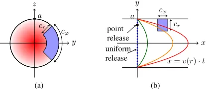
Fig. 1. System model geometry (a) in the cross-section, and (b) along the axis. The red shading in (a) reflects the flow velocity which is maximum in the center and vanishes at the boundary. The corresponding parabolic shape, x=v(r)·t, on which released particles reside when not diffusing after a uniform release, is sketched in (b) for three different time instances. Point and uniform transmitter release are shown as black dot and as a blue line, respectively.
II. SYSTEMMODEL ANDPRELIMINARIES
A. System Model
We consider a straight impermeable cylindrical duct of
infinite axial extent and radius a which can be described
in cylindrical coordinates by the points (x, r, ϕ), where
x ∈ (−∞,∞) is the axial position, r ∈ [0, a] is the radial
distance, and ϕ ∈ (−π, π] is the azimuth angle. The duct
is filled with a fluid of viscosity η that is subject to steady
laminar flow in the x-direction where the flow velocity v(r)
is a function of r only and is given by a parabolic function;
see Fig. 1.
We consider a transmitter (TX) that releases NTX molecules
via on-off keying (OOK) either 1) uniformly and randomly
distributed over the cross section at x = 0, or 2) from the
point(0, r0, ϕ0). Moreover, we assume a transparent receiver
(RX) specified by the points (x, r, ϕ) satisfying |x−d| ≤
cx/2, a−cr≤r≤a,|ϕ| ≤cϕ/2, i.e., the receiver is mounted
on the duct wall with axial TX-RX distance given byd, radial
extentcr, and spanning an angle ofcϕ (see Fig. 1). Detection of the OOK symbolsa[k]∈ {0,1} is performed based on the
number of observed particles Nob(t)by applying a threshold
ξ∈ {0,1, . . . , NTX}:
ˆ a[k] =
(
0, Nob(t0+kT)< ξ 1, Nob(t0+kT)≥ξ,
(1)
where t0 is a detection delay andaˆ[k] is the detected OOK
symbol in the k-th symbol interval of length T, i.e., for OOK
1/T is the data rate.
We model the particle release from the TX as instantaneous and the released particles are transported by the fluid flow and Brownian motion. For simplicity, we assume that particles do not interact with each other nor influence the flow field. Because of their small size, other forces such as gravity acting on the particles are negligible [7].
B. Preliminaries
In molecular communication, information is conveyed by mass transfer. Mass transfer in fluids is mediated by flow
and Brownian motion which is referred to as advection and
diffusion, respectively. Thereby, mass transfer can be described
by a time-varying spatial probability density function (PDF) p(r;t)which can be interpreted as a normalized concentration wheredV·p(r;t)gives the average fraction of particles within the differential volumedV atrat timet. The PDFp(r;t)can be found as the solution to the following partial differential equation (PDE), which we will also refer to as the advection-diffusion equation [7, Eq. (5.22)]
∂tp=D∇2p− ∇ ·pv, (2) where∂tp=∂t∂pdenotes the partial derivative ofpwith respect
tot and∇is the Nabla operator. Moreover,D is the diffusion
coefficient andv(r)is the velocity vector at pointr.
To solve (2), we need to know the velocity field v(r). In
general, the velocity field can be obtained by solving the Navier-Stokes equation, which provides a fundamental description of flow by relating the velocity field to the local pressure [7, Ch. 2]. Applied to rigid and straight channels with no-slip boundary conditions, i.e., where the velocity at the boundary is zero, and subject to pressure-driven flow in the steady-state, the velocity profile is referred to asPoiseuille flow[7, Ch. 3].
Thereby, assuming aNewtonian fluid, i.e., a fluid which can
be described by the viscosityη, we obtain [7, Eq. (3.32)]
v(r) = 2veff
1−r
2
a2
, (3)
whereveff is the mean velocity in the channel and is a function
of the applied pressure gradient∂xP. In particular,veff can be
obtained as [7, Eq. (3.34)]
veff= |∂xP|a
2
8η .
We note that the maximum velocityvmax= 2veff occurs at
the center and can be found usingr= 0 in (3).
An important parameter is the P´eclet number, which gives an estimate of the importance of diffusion over advection. This dimensionless number is defined as [6, Eq. (4.6.8)]
Pe = veffa
D , (4)
when considering the duct radius a as the length scale of
interest. Intuitively,Pe∈[0,∞)increases and decreases when
veff andD increase as the importance of particle transport by
flow and diffusion becomes more relevant, respectively.
III. ANALYSIS OF THEDUCTCHANNEL
The advection-diffusion equation (2) for the environment in Fig. 1 simplifies to the following PDE:
∂tp=D∇2p−v(r)∂xp, (5)
for t > 0 because the velocity field is independent of the
axial position. At the boundary r = a, ∂rp = 0 has to
hold and p(x, r, ϕ; 0) is initially given by δ(x)/(πa2) and δ(x)δ(r −r0)δ(ϕ −ϕ0)/r for uniform and point release, respectively. Eq. (5) is still difficult to solve in general because
of the nonlinear velocity (3) and the inherent coupling of p
cross-sectional diffusion and the non-uniform flow profile have
averaged out. We will refer to this behavior as the dispersion
regime. Trivially, this regime includes the special case where
veff → 0, i.e., when there is pure diffusion. Another special
case where (5) can be solved is when D→0, i.e., when we
are in theflow-dominated regime.
For each of these regimes, we seek the time-dependent observation probability
Pob(t) = Z
VRX
p(x, r, ϕ;t) dVRX, (6)
where VRX is the RX volume. We will also refer toPob(t)as theimpulse response of the molecular communication channel.
The impulse response is a fundamental characteristic of the molecular communication channel as it determines the mean Nob(t)of the received signal [2]Nob(t)
Nob(t) =NTX ∞
X
k=0
a[k]Pob(t−kT) +Nn, (7)
whereNn is external noise. We note that in generalNob(t)is a binomial random variable which can be approximated by a
Poisson random variable of mean Nob(t)[2]. Based on this
assumption also the symbol error rate (SER) can be determined which, as performance measure, we will evaluate in Section IV.
A. Dispersion Regime
Dispersion is the result of the interaction of cross-sectional diffusion and the non-uniform advection due to the flow profile. This interaction can lead to a particle distribution that is uniform in each cross-section, i.e., the spatial PDF can be written as p(x, r, ϕ;t) = p(x;t)/(πa2). In this regime, the particle
distribution does depend only on the initial x-position, i.e.,
there is no difference for point and uniform release. This behavior occurs if [6, Chapter 4.6]
Pe4d
a, (8)
e.g., when the TX-RX distance is large, the diffusion coefficient is large, or the duct radius is small. Naturally, this includes the special case of pure diffusion where flow is not present. If (8) is satisfied, (5) can be written as the following 1D advection-diffusion equation [6, Eq. (4.6.30)]
∂tp=Deff∂x2p−veff∂xp, (9)
with effective diffusion coefficientDeff and mean velocity veff.
For an instantaneous uniform release at x= 0, the solution to
(9) is given by
p(x, r, ϕ;t) = 1
πa2 ×
1
√4πD efftexp
−(x−vefft)
2
4Defft
, (10)
where1/(πa2)is the cross-sectional distribution in the r- and ϕ-directions.
Following [11, Eq. (26)], the Taylor-Ariseffective diffusion
coefficientDeff is obtained as [6, Eq. (4.6.35)]
Deff=D
1 + 1
48Pe
2. (11)
We note that in general Deff > D and moreover Deff
D when D is decreased to very small values, which by (4)
increases Pe. However, by (8), decreasing D comes at the
expense of a larger required distance for dispersion to take place. In fact, we can rearrange (8) as
D a
2
·veff
4d , (12)
which approximates the minimum diffusion coefficient required
for dispersion to occur. For small and largeD, we can neglect
the first and second parts in the sum on the right-hand side of (11), respectively.
The observation probability obtained by integrating (10) over the receiver volume is given by (6)
Pob,d(t) = ARX
a2 ×
Q
d
−cx/2−vefft 2Defft
−Q d+c
x/2−vefft 2Defft
, (13)
where Q(·)is the Gaussian Q-function and ARX =cϕ/(2π)·
(2acr−c2r)is the surface area of the RX in the cross section. It is of interest to derive the time at whichPob,d(t)attains its maximum as this may serve as design guideline for the symbol interval length. As maximizing Pob,d(t)with respect
tot is cumbersome, we resort to maximizing (10) forx=d,
which yields
tmax=Deff v2
eff − 1 +
s 1 + v
2
eff
D2
eff
d2 !
. (14)
In this approximation, the peak height follows aspmax =
Pob,d(tmax). We note that because of diffusiontmax< d/veff,
whered/veff is the time when particles moving with the mean
velocity will reach the RX.
B. Flow-dominated Regime
In this subsection, we directly determine the observation probability Pob,f(t) = Pob(t) by neglecting diffusion and without resorting to (6).
1) Uniform Release: First, we assume a uniform release
at x = 0. In this case, all particles will lie on the surface
of a paraboloid that extends along the axis over time and exhibits rotational symmetry. Thereby, the marginal distribution in the cross-section, i.e., for ther- andϕ-coordinates, remains
uniform because the flow is in thex-direction. The geometric
shape is given by x= v(r)·t, cf. Fig. 1. Hence, the time
t when the points (x, r, ϕ) lie on the paraboloid is simply
given by t=x/v(r). From this, we also obtain the following auxiliary relationship:
rt(x) =a·
r
1− x
2vefft, (15)
which is obtained by re-arranging (3).
atx= 0, the observation probabilityPob,f(t)can consequently be written as Pob,f(t) = cϕ/(2π)·(ro2−r2i)/a2. Variables ri(t)andro(t)depend on how the paraboloid intersects with the RX volume. In fact, there are three scenarios, which are
shown in Fig. 1b for the x-y-plane. In the first case, the
paraboloid has not yet reached the RX, cf. the green line
in Fig. 1b. The first intersection occurs at t =t1 when the
paraboloid reaches the points (x=d−cx/2, r =a−cr, ϕ) whereϕ∈[−cϕ/2, cϕ/2]. In the second case, for t1< t < t2, the paraboloid intersects with the RX at ri(t) =a−cr and ro(t) =rt(d−cx/2), cf. the orange line in Fig. 1b. Timet2 is characterized by the paraboloid intersecting with the RX at the points(d+cx/2, a−cr, ϕ)whereϕ∈[−cϕ/2, cϕ/2]. The last case occurs for t≥t2, cf. the red line in Fig. 1b. In this case, we have ri(t) =rt(d−cx/2) andro(t) =rt(d+cx/2).
Now, we only requiret1and t2 in order to obtain the impulse
response. Fromx=v(r)·t and (3), we obtain
t1,2=
d∓cx/2
2veff(1−(1−cr/a)2) (16) In summary, the impulse response in the flow-dominated regime following a uniform release can be written as
Pob,f(t) =
0, t≤t1
1
a2ARX− cϕ
2π
d−cx/2
2vefft
, t1< t < t2
cϕ
2π· cx
2vefft, t≥t2.
(17)
Pob,f(t)is maximized fort=t2. Also, at timet=t2/αthe fraction α∈(0,1]ofPob,f(t2) can be observed. The tail of the impulse response decays only polynomial with time, which may give rise to significant ISI in molecular communication systems.
2) Point Release: For a point release withr0∈[a−cr, a] and ϕ0 ∈ [−cϕ/2, cϕ/2], i.e., when the TX coordinates are
within the r- and ϕ-coordinates of the RX, we observe all
particles with certainty if d−cx/2≤v(r0)t≤d+cx/2, i.e., the impulse response is given by
Pob•,f(t) = rect v(r
0)t−d cx
, (18)
where rect(x) = 1 if −1/2 ≤ x≤1/2 and zero otherwise.
When the release point isnotwithin the r- andϕ-coordinates
of the RX then the impulse response is zero for all times.
Eqs. (17) and (18) are intuitively valid when D→0. More
generally, the solution is applicable whenPed/a[6], e.g.,
when the duct radius is large or the TX-RX distance is small. We note that (17) and (18) still give the observation
probability ∈ [0,1] even though the flow is deterministic, i.e., with probability Pob(t)and 1−Pob(t)each of theNTX particles can be independently and cannot be observed within
the RX volume at time t, respectively. The reason for this
is that for both uniform and point release the initial particle position can be understood as independently and uniformly random distributed within the available TX area (the whole cross section or one point).
IV. NUMERICALEVALUATION
By using particle-based simulation, we validate our derived analytical expressions and explore those regimes for which mathematical analysis is not readily accomplished. Thereby, unless explicitly stated otherwise, we employ the following physical parameter values. As diffusion coefficient we choose
D = 10−10m2/s which is a reasonable estimate for small
proteins [6]. Two values for the duct radius a= 10µm and
a = 200µm are considered, which is reasonable for small capillaries [6] and microfluidic ducts [7], respectively. Thereby,
two TX-RX distances are considered with valuesd= 200µm
andd= 800µm. Moreover, we choose the receiver dimensions ascx=a/2,cr=a/2,cϕ=π/2, i.e., the receiver size scales with the duct radius. The microscopic simulation time step is set to∆t= 10−3s. The fluid flow mean velocity is assumed to be veff= 1 mm s−1, which is reasonable for small capillaries [6].
For a = 10µm, for D = 10−10m2/s, we obtain D
eff = 2.1×10⁻⁸m2/s, which is a value otherwise unattainable for
the diffusion coefficient of small proteins [6]. Fora= 50µm
and a = 200µm, for D = 10−10m2/s and d= 800µm by
(12) Deff is not meaningful anymore, cf. Fig. 2.
We show in Fig. 2 (adapted from [6]) the considered parameter values in terms of the P´eclet number and the ratio of the TX-RX distance to the duct radius. In particular, we have shaded the two regimes for which the obtained analytical results from Section III are expected to be applicable. Eq. (8) separates these two regimes and is shown as black line. The derived analytical results are valid for parameter values well within the dispersion or the flow-dominated regime. However, the analytical results cannot be expected to be accurate close the boundary set by (8). For the two duct radiia= 10µm,200µm
and the two TX-RX distancesd= 200µm,800µm, we show
[image:5.612.55.302.317.381.2]the resulting four combinations ofd/aandPeas black dots in
Fig. 2. We see that the two scenarios fora= 10µmlie close to the boundary of both regions. These parameter values have been chosen such that simulations can reveal the deviations from
either regime. On the other hand, the scenarios fora= 200µm
lie well within the flow-dominated regime and we expect no deviations from the developed theory. We note that changing
the duct radiusaaffects bothd/aandPewhereas a change in
dinfluences onlyd/a. Considering the parameter values chosen
in this paper, from Fig. 2, we can conclude that the dispersion regime is most applicable for small microscale ducts. On the other hand, we also see that there is a large set of parameters for which the flow-dominated regime is more appropriate, especially for medium to large ducts.
To gain a basic understanding of the particle evolution towards dispersion, in Fig. 3, we show three snapshots of the particle positions corresponding to three different time instances and distinguished by different colors following a
uniform release at t = 0. In particular, we plot r2 over x
motivated by the fact that the marginal distribution inr2 of
a uniform distribution within a circular disk is uniform. As
a side effect, for the flow-dominated regime from (15), r2
log10(Pe)
log10(d/a)
dispersion
flow-dominated
0.6 2
d= 200µm
d= 800µm a= 10µm
a= 200µm
Fig. 2. Sketch of regions of different transport regimes. Adapted from [6]. All four simulation scenarios are shown as black dots. Fora= 10µm, we havePe = 100andd/a= 20,80. Fora= 200µm, we havePe = 2000
andd/a= 1,4.
0 500 1,000 1,500
0 50 100
x[µm]
r
2[µ
m
[image:6.612.322.553.50.338.2]2]
Fig. 3. Snapshot of particle positions for a = 10µm and at t = 0.02,0.2,0.8 safter uniform release atx= 0andt= 0shown in different colors and starting from left to right, respectively. In total,NTX= 103are
released.
t is shown as a blue line. Furthermore,a= 10µm such that
according to Fig. 2, dispersion occurs for xin the vicinity of
d= 800µm. For the largest time shown,t= 0.8 s, the red lines show the standard deviation positions vefft±√2Defftfrom the
mean when assuming the Gaussian distribution in (10) due to dispersion. For small times, e.g.,t= 0.02 s, the particles follow the parabolic profile (15) closely. For slightly larger times, e.g., t = 0.2 s, the particles start to spread because of diffusion.
For large times, e.g., t = 0.8 s, particles become uniformly
distributed along the r2 dimension within the duct due to
dispersion. We note that forveff= 1 mm s−1, att= 0.2 sand
t= 0.8 s, the mean particle position has arrived atd= 200µm andd= 800µm, respectively. In summary, at small times after the release the flow-dominated regime and at large times after the release the dispersion regime accurately model the actual behavior.
In Figs. 4a and 4b, we show the impulse response fora=
10µmanda= 200µm, respectively. In each case, we consider bothd= 200µmandd= 800µmas well as uniform and point release. For the point release, the position (0,0.75a,0) was chosen such that particles can arrive at the receiver when not diffusing. We simulate the impulse responses and investigate which of the developed analytical models provides the best fit in each case.
In Fig. 4a, for comparison, bothPob,d(t)(applicable for both point and uniform release) in (13) andPob,f(t)(applicable only for uniform release) in (17) are shown. Thereby, for Pob,d(t), the peaks via (14) are also highlighted with large dots. When d= 200µm, the simulated impulse response following a point release is significantly larger than that for a simulated uniform release. In this case, both simulated impulse responses neither matchPob,d(t)norPob,f(t). However, especially considering the long-time behavior, e.g., for t >0.5 s, the simulated data points tend to be better described byPob,d(t)than byPob,f(t). For d = 800µm, the deviations of the simulated impulse
0 0.5 1 1.5 2
0 0.5 1
·10−2
d=
200
µm
d= 800µm
time ins
fraction
of
particles
Pob,f(t)
Pob,d(t)
sim. unif. sim. point peak
(a)
0 0.5 1 1.5 2
0 0.5 1
·10−1
d=
200
µm
d= 800µm
d= 200µm
time [s]
fraction
of
particles
Pob,f(t)
0.1·Pob•,f(t)
sim. unif.
0.1·sim. point peak
[image:6.612.86.263.54.136.2](b)
Fig. 4. Impulse responses for (a)a= 10µm, and (b)a= 200µm. Simulation results are shown for both uniform and point release. For (b), additionally the simulated and analytical impulse responses due to a point release are scaled by the constant factor0.1for a better visualization. Simulation results are for NTX= 106.
responses for point and uniform release from Pob,d(t) are
much smaller and the dispersion regime provides a much better fit despite the fact that (8) is not strictly satisfied, cf. Fig. 2. This is consistent with the green particle cloud in
Fig. 3 which appears uniform inr2. ComparingP
ob,f(t)and Pob,d(t), we see that the peak ofPob,f(t)is larger and smaller than that ofPob,d(t)whendis small and large, respectively. For larger times, e.g., fort >0.75 s,Pob,f(t)for d= 200µm andPob,f(t)ford= 800µm coincide as expected from (17) which is independent ofdfort > t2. In conclusion, parameter values close to the boundary in Fig. 2 can still be applicable for the dispersion model.
In Fig. 4b, Pob,f(t)in (17) andPob•,f(t)in (18) are shown.
For the former, the peak times t2 are highlighted. For both
uniform and point release, simulation results are also shown. By Fig. 2, the dispersion approximation is not applicable in this scenario and for clarity is not shown. Considering the
point release, the simulated curve ford= 200µm matches the
rectangular shape of P•
ob,f(t)in (18) reasonably well. On the
other hand, for d= 800µm, the simulated impulse response
[image:6.612.79.270.191.246.2]0.2 0.4 0.6 0.8 1 10−5
10−3 10−1
200µm
400µm
600µm 800µm
symbol interval ins
SER
Fig. 5. Symbol error rate as a function of the symbol interval length for d= 200,400,600,800µm. Parameters are chosen asNTX= 104,Nn= 10.
a small deviation because of residual particles close to the RX when most particles have already passed. Comparing the impulse responses for point release and uniform release, we find that the tail of the impulse response strongly depends on the initial distribution. There can be considerable ISI, especially when a fraction of the particles is released close to the duct wall. However, as long as the RX can be reached by the particles, an initial release close to the center of the duct might reduce ISI. Comparing Figs. 4a and 4b, we see that the channels behave completely different when the duct radius is changed from a = 10µm to a = 200µm. We note that for both uniform and point release the peak values of the impulse responses in Fig. 4a are at least by an order of magnitude smaller than in Fig. 4b. Moreover, for uniform and point release the simulated impulse responses in Fig. 4a decay faster and slower from their peak values than those in Fig. 4b, respectively.
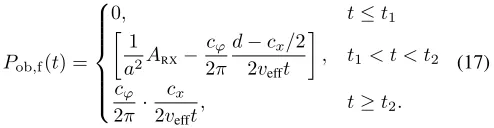
In Fig. 5, we show the average SER for OOK modulation of maximally 8 interfering symbols and threshold detection of the detected number of transmitted particles as a function of the symbol interval length using the analytic impulse response in (17) for the flow-dominated regime. The curves
are parameterized by the TX-RX distanced, which is varied
from200µmto800µm. As detection time offset, i.e., as delay,
t0 = t2 is chosen and an average of 10 noise molecules is
assumed. For each considered symbol interval and TX-RX
distance, the minimum SER over the threshold ξis found by
full search. In general, the SER decreases for increasing T
at the expense of decreasing the data rate1/T. However, for
moderate to large distances, e.g., d= 800µm, the SER does
not decrease significantly even if the symbol interval is taken
very large, e.g., T = 1 s, because of severe ISI, cf. Fig. 4b.
The supported distance for a maximally tolerated SER could potentially be increased by adapting the injection mechanism as can drastically be seen by the rectangular-shape impulse response for a point release in Fig. 4b. On the other hand, additional processing of the received signal before detection such as differentiating the received signal might also enhance the performance.
V. CONCLUSION
Dispersion generalizes the concept of diffusion which is crucial for signal propagation in molecular communication.
Thereby, a non-uniform flow can be accounted for by an ef-fective diffusion coefficient. This efef-fective diffusion coefficient can be multiple orders of magnitude larger than the molecular diffusion coefficient. However, this description relies on a large TX-RX distance. On the other hand, there are many practical scenarios at the microscale that fall within a flow-dominated regime where dispersion is insignificant. In this regime, the initial release pattern drastically influences ISI. For a given duct radius either regime can be applicable depending on the TX-RX distance and the P´eclet number.
REFERENCES
[1] N. Farsad, H. B. Yilmaz, A. Eckford, C. B. Chae, and W. Guo, “A com-prehensive survey of recent advancements in molecular communication,”
IEEE Commun. Surv. Tutorials, vol. 18, no. 3, pp. 1887–1919, 2016.
[2] A. Noel, K. C. Cheung, and R. Schober, “Optimal receiver design for diffusive molecular communication with flow and additive noise,”IEEE Trans. Nanobioscience, vol. 13, no. 3, pp. 350–362, Sep. 2014.
[3] W. Wicke, A. Ahmadzadeh, V. Jamali, H. Unterweger, C. Alexiou, and R. Schober, “Molecular communication using magnetic nanoparticles,”
arXiv:1704.04206, Accept. for Present. IEEE WCNC 2018.
[4] K. V. Srinivas, A. W. Eckford, and R. S. Adve, “Molecular communication in fluid media: The additive inverse Gaussian noise channel,”IEEE Trans. Inf. Theory, vol. 58, no. 7, pp. 4678–4692, Jul. 2012.
[5] N. R. Kim, A. W. Eckford, and C. B. Chae, “Symbol interval optimization for molecular communication with drift,”IEEE Trans. Nanobioscience,
vol. 13, no. 3, pp. 223–229, Sep. 2014.
[6] R. F. Probstein,Physicochemical Hydrodynamics: An Introduction. John
Wiley & Sons, Feb. 2005.
[7] H. Bruus,Theoretical Microfluidics, 1st ed. Oxford University Press,
Nov. 2007.
[8] M. Kuscu and O. B. Akan, “Modeling convection-diffusion-reaction systems for microfluidic molecular communications with surface-based receivers in internet of bio-nano things,”PLoS One, vol. 13, no. 2, p.
e0192202, 2018.
[9] L. Felicetti, M. Femminella, and G. Reali, “Simulation of molecular sig-naling in blood vessels: Software design and application to atherogenesis,”
Nano Commun. Networks, vol. 4, no. 3, pp. 98–119, Sep. 2013.
[10] G. I. Taylor, “Dispersion of soluble matter in solvent flowing slowly through a tube,”Proc. R. Soc. Lond. A, vol. 219, no. 1137, pp. 186–203,
Aug. 1953.
[11] R. Aris, “On the dispersion of a solute in a fluid flowing through a tube,”
Proc. R. Soc. Lond. A, vol. 235, no. 1200, pp. 67–77, Apr. 1956.
[12] P. He, Y. Mao, Q. Liu, P. Li, and K. Yang, “Channel modelling of molecular communications across blood vessels and nerves,” inProc. IEEE ICC 2016, May 2016, pp. 1–6.
[13] Y. Chahibi, M. Pierobon, and I. F. Akyildiz, “Pharmacokinetic modeling and biodistribution estimation through the molecular communication paradigm,”IEEE Trans. Biomed. Eng., vol. 62, no. 10, pp. 2410–2420,
Oct. 2015.
[14] A. O. Bicen and I. F. Akyildiz, “System-theoretic analysis and least-squares design of microfluidic channels for flow-induced molecular communication,”IEEE Trans. Signal Process., vol. 61, no. 20, pp. 5000–
5013, Oct. 2013.
[15] Y. Sun, K. Yang, and Q. Liu, “Channel capacity modelling of blood capillary-based molecular communication with blood flow drift,” inProc. ACM NanoCom 2017, 2017, pp. 19:1–19:6.
[16] A. O. Bicen, J. J. Lehtom¨aki, and I. F. Akyildiz, “Shannon meets Fick on the microfluidic channel: diffusion limit to sum broadcast capacity for molecular communication,”IEEE Trans. Nanobiosci., vol. 17, no. 1,
pp. 88–94, 2018.
[17] H. Unterweger, J. Kirchner, W. Wicke, A. Ahmadzadeh, D. Ahmed, V. Jamali, C. Alexiou, G. Fischer, and R. Schober, “Experimental molecular communication testbed based on magnetic nanoparticles in duct flow,”arXiv preprint arXiv:1803.06990, 2018.
[18] O. Levenspiel,Chemical reaction engineering, 3rd ed. John Wiley &
[image:7.612.90.257.50.176.2]