Phase field modelling of surfactants in multi phase flow

warwick.ac.uk/lib-publications

Manuscript version: Author’s Accepted Manuscript

The version presented in WRAP is the author’s accepted manuscript and may differ from the published version or Version of Record.

Persistent WRAP URL:

http://wrap.warwick.ac.uk/126567

How to cite:

Please refer to published version for the most recent bibliographic citation information. If a published version is known of, the repository item page linked to above, will contain details on accessing it.

Copyright and reuse:

The Warwick Research Archive Portal (WRAP) makes this work by researchers of the University of Warwick available open access under the following conditions.

Copyright © and all moral rights to the version of the paper presented here belong to the individual author(s) and/or other copyright owners. To the extent reasonable and

practicable the material made available in WRAP has been checked for eligibility before being made available.

Copies of full items can be used for personal research or study, educational, or not-for-profit purposes without prior permission or charge. Provided that the authors, title and full

bibliographic details are credited, a hyperlink and/or URL is given for the original metadata page and the content is not changed in any way.

Publisher’s statement:

Please refer to the repository item page, publisher’s statement section, for further information.

Oliver R. A. Dunbar

California Institute of Technology,

1200 E. California Blvd. MC 131-24, Pasadena, CA 91125, USA

[email protected]

Kei Fong Lam

Department of Mathematics,

The Chinese University of Hong Kong,

Shatin, N.T., Hong Kong

[email protected]

Bj¨orn Stinner

Mathematics Institute and Centre for Scientific Computing,

University of Warwick, Coventry CV4 7AL, United Kingdom

[email protected]

October 1, 2019

Abstract

A diffuse interface model for surfactants in multi-phase flow with three or more fluids is derived. A system of Cahn–Hilliard equations is coupled with a Navier–Stokes system and an advection-diffusion equation for the surfactant ensuring thermodynamic consistency. By an asymptotic analysis the model can be related to a moving boundary problem in the sharp inter-face limit, which is derived from first principles. Results from numerical simulations support the theoretical findings. The main novelties are centred around the conditions in the triple junctions where three fluids meet. Specifically the case of local chemical equilibrium with respect to the surfactant is considered, which allows for interfacial surfactant flow through the triple junctions.

2010 Mathematics Subject Classification: Primary 35R37; Secondary 76T30, 35R01, 35C20, 76D45.

Keywords: Surfactant; diffuse interface; adsorption isotherm; triple junction; thermodynamic consistency.

1

Introduction

Surfactants (surface active agents) are chemicals that, when dissolved in a system of multiple im-miscible fluids, tend to form layers at the fluid-fluid interfaces and thus reduce the surface tension.

Such manipulation is exploited in nature and industry, and we refer to [60, 72] for overviews of the vast applicability of surfactants and to [20, 46, 51, 52, 67] for specific applications involving more than two phases.

Several approaches to such problems based on the representation of the interfaces by hypersur-faces (here calledsharp interface models) are available, among which we mention interface track-ing methods [44, 47, 53, 58, 59, 75], volume-of-fluid methods [5, 42, 45, 61], and ALE methods [10, 32, 80], see also the books [14, 38]. In general, the fluid-fluid interfaces undergo changes of topology, which may manifest as the breakup of droplets, pinching, coalescence, or cusp formation or tip-streaming driven by Marangoni forces. To overcome the analytical and numerical complica-tions associated to such events one can turn to interface-capturing methods such as level-set methods [3, 71, 78, 79], ordiffuse interfaceapproaches, which comprise thephase field methodology.

In this work we address the phase field modelling of surfactant dynamics in multi-phase flow with more than two fluids. The classical description of fluid-fluid interfaces with hypersurfaces is replaced by one with thin transition layers of a thickness that scales with a small parameterε. Within these thin layers, some form of microscopic mixture of the macroscopically immiscible fluids is

allowed. One then introduces order parameters or phase field variables that serve to distinguish

between the bulk phases, where the phase fields are close to constants, and the interfacial layers, across which the phase fields change values quickly but smoothly.

The notion of diffuse interfaces dates at least back to van der Waals [77]. In [43], model H

couples a Cahn–Hilliard equation with a Navier–Stokes system. Subsequent efforts have been di-rected to extend this type of model with regards to non-matched densities [57], divergence-free mixture velocities [25], thermodynamic consistency [1, 40], and flows with more than two fluids [9, 15, 26, 27, 48, 49, 50]. Regarding the inclusion of surfactants we refer to [30, 55, 56, 74, 76, 81], all of which are restricted to two fluids.

Our phase field model builds on [33], where surfactants in two-phase flow are studied within

a free energy framework. The focus of this study is on theinstantaneous adsorptionregime when

the adsorption-desorption process between interfacial surfactant and bulk surfactant in the adjacent sublayers occurs at a much faster timescale relative to other diffusive or convective processes in the

system. The relation between interfacial and bulk surfactant is commonly described byisotherms

[28]. Within a free energy framework this local chemical equilibrium condition can be expressed as an equality of the chemical potentials of the (surfactant dependent) interfacial and bulk free energies [24, 65].

from the adjacent interfaces is zero and the interfacial surfactant chemical potentials match up at the triple junction.

Under some convexity assumptions on the bulk and surface free energies the local chemical equilibrium assumption enables us to introduce a single continuous (chemical) potential field in which the balance laws for the bulk and interfacial surfactants can be expressed, as can the surfactant dependent surface tensions. These coupled equations can be formulated in a distributional form in the context of sharp interface models. Here, we can follow the lines of [6], which covers the two-phase case and can be extended to account for triple junctions. This form allows for an incorporation into a phase field model with thin layers representing the interfaces. It is achieved by smoothing the distributions associated with the bulk domains and interfaces in terms of the phase field variables. We refer to [33, 54, 64, 73, 74] for the ideas and to [2, 21, 29] for rigorous analytical investigations in the two-phase case.

One of the challenges in the case of multiple fluids is to choose suitable smoothing functions such that (a) the interfacial surfactant equation for each specific fluid-fluid interface is consistently approximated and (b) the conditions in the triple junctions are consistently approximated, as the diffuse interface thickness converges to zero. A key ingredient to solve this problem are phase field potentials that avoidthird phase contributionsat interfaces, i.e., in the interfacial layer between two phases only the phase field variable associated with these phases are present [15, 16, 17, 35, 70]. This allows for a precise localisation of fields and functional dependencies that are supposed to be present at a specific interface or a triple junction only.

It is also desirable that the smoothing leads to a model with good structural properties such as thermodynamic consistency and a solenoidal velocity field, which are beneficial for numerical approximations. As in [33] our model for the multi-phase flow is based on [1]. This approach is extended to account for multiple fluids. As in [40] it assumes that, within the interfacial layers where the fluids mix, inertia and kinetic energy due to the motion of the constituent fluids relative to the gross motion of the mixture is negligible. Often, the mass-averaged velocity is chosen to define the gross motion [39, 48, 49, 50, 57]. But taking the volume-averaged velocity as in [9, 25, 26, 27] leads to a divergence-free velocity field. Moreover, we can ensure that thecalibration of our phase field model is convenient in the following sense: Parameters (fluid densities, viscosities, surfactant diffusivities, etc) and relations in the sharp interface model (dependence of the surface tension on the surfactant, etc) directly reappear in the phase field model, no adjustment or rescaling is required.

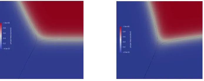
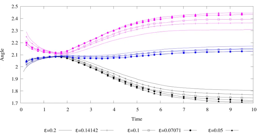
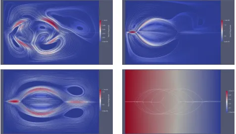
in the small interfacial thickness parameterεis presented in Section 4. As one of the main novelties we show that the conditions for the surfactant in the triple junction indeed are obtained in the sharp interface limit. The conditions at the fluid-fluid interfaces have been analysed in [33], to which the present multi-phase case arguably reduces if the third phase contributions, which were mentioned above, can be avoided. However, the details are presented as they are required for the analysis around the triple junctions. We have performed some numerical simulations on a qualitative level in order to validate and support the theoretical results of the asymptotic analysis, see Section 5.

2

Sharp interface model

In deriving the free boundary problem, which we intend to approximate with a phase field model, we extend [33] by accounting for multiple phases. This implies that the conditions at points where several phases meet have to be discussed. A general study of balance equations in three phase systems including bulk, surface, and triple line fields is presented in [13]. We re-state some of the theory in order to introduce our notation and to define our specific closing conditions.

2.1

Setting

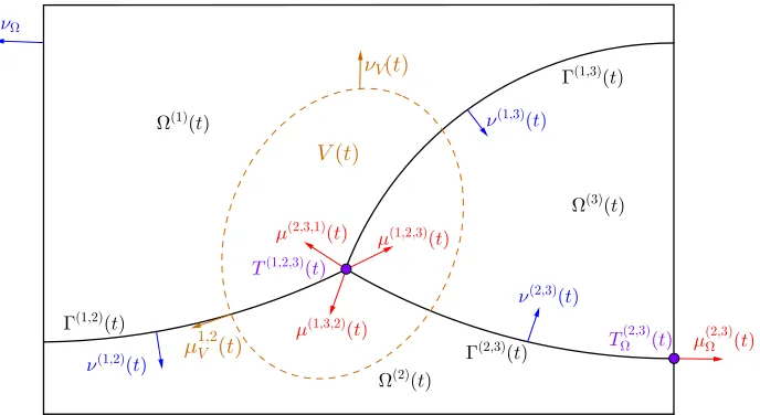
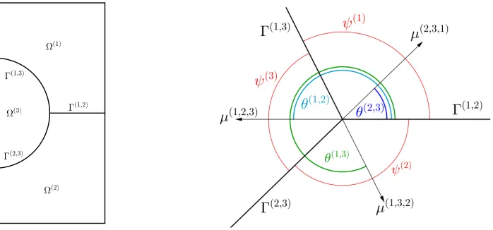
LetΩ ⊂ _Rd_{, d ∈ {2,3}, be a bounded domain and I = [0, T), T ∈ (0,∞]be a time interval. We}

assume thatΩis partitioned by moving hypersurfacesΓ(i,j)_{(t)intoM time-dependent open}

subdo-mainsΩ(k)(t), i, j, k ∈ {1, . . . , M}. Intersections of three hypersurfaces are denoted byT(i,j,k)(t)

and form triple points (d = 2) or form triple lines (d = 3) ending at quadruple pointsQ(i,j,k,l)_(t),

i, j, k, l∈ {1, . . . , M}. For simplicity, with regards toT(i,j,k)(t)we will only talk abouttriple

junc-tions in the following. Similarly, on the external boundary∂Ωthere are (possibly moving) triple

points or linesT_Ω(i,j)(t)with quadruple pointsQ(_Ωi,j,k)(t)ifd= 3. The unit normal onΓ(i,j)_(t)

point-ing out ofΩ(i)(t)intoΩ(j)(t)is denoted byν(i,j)(t), and byνΩwe denote the outward unit normal

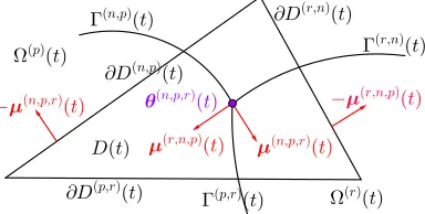
on∂Ω. For the conormal of Γ(i,j)_{(t) atT}(i,j,k)_{(t)pointing into Ω}(k)_{(t)we write µ}(i,j,k)_{(t), and we}

writeµ(_Ωi,j)(t)for it on∂Ω. Figure 1 is a sketch of a configuration we have in mind.

The whole configuration is transported by a continuous velocity fieldv : [0, T)×Ω→ _Rd_{. For}

the interfaces this implies that

[v(t)]j_i =0, u(i,j)(t) :=v(t)·ν(i,j)(t) onΓ(i,j)(t), (2.1) where [·]j_i = (·)(j) _−(·)(i) _{stands for the jump from domainΩ}(i)_{(t) into Ω}(j)_{(t) across the}

inter-face Γ(i,j)(t), and u(i,j)(t) is the (scalar) normal velocity of Γ(i,j)(t) in direction ν(i,j)(t). In two dimensions, we define the velocity of the triple pointT(i,j,k)_(t)as

u(i,j,k)(t) :=v(t)|_T(i,j,k)_(t).

In three dimensions, the triple line T(i,j,k)_{(t) is a space curve. In every point x ∈ T}(i,j,k)_{(t), let}

one-Figure 1:Illustration of the setting described in Section 2.1.

dimensional tangent spaceTxT(i,j,k)(t)ofT(i,j,k)(t), i.e., with any unit tangent vectorsτ(i,j,k)(x, t)

ofT(i,j,k)_(t)inx

P_(T(i,j,k)_(t))⊥(x) =I −τ(i,j,k)(x, t)⊗τ(i,j,k)(x, t).

We define the (vector-valued) normal velocity of the triple line by

u(i,j,k)(t) := P_(T(i,j,k)_(t))⊥v(t) onT(i,j,k)(t). (2.2)

Notice that, in two dimensions, P_(T(i,j,k)_(t))⊥ reduces to the identity map, and so (2.2) becomes u(i,j,k)_{(t) = v(t)atT}(i,j,k)_{(t)as defined before. We may thus use (2.2) also in the cased = 2. Let}

us remark thatu(i,j,k)(t)is an intrinsic field that describes instantaneous changes to the geometry of T(i,j,k)_{(t) in time, where we refer to [6], Sec. 2.1 for more details. In the following, we will}

often omit the dependence on timetof hypersurfaces, triple junctions, and related objects for better readability.

The surface derivative and divergence along the hypersurfaceΓ(i,j) _{are denoted by ∇}

Γ(i,j) and

∇_Γ(i,j)·, respectively. Further notation concerns the material derivative for a fieldw: [0, T)×Ω→R,

∂_t•(v)w:=∂tw+v· ∇w, (2.3)

where we remark that this operator is well-defined for fields restricted to a hypersurfaceΓ(i,j). For such fieldswwe also consider the normal time derivative,

∂_t◦(u(i,j))w:= ∂tw+u(i,j)ν(i,j)· ∇w, (2.4)

and note that

Some identities such as a transport identity on evolving surfaces and integration by parts formula on surfaces are stated in the Appendix. Byκ(i,j) _{we denote the mean curvature vector ofΓ}(i,j)_.

The sharp interface model will be derived by stating balance equations and considering the free energy on so-calledarbitrary material test volumes. By this we mean setsV(t)⊂ Ωof points that move with velocityv(t)in the domain at least for a small open time interval so that derivatives with respect to time can be considered. Though these sets indeed are fairly arbitrary we make some as-sumptions as specified below. These could be dropped at the expense of substantially more detailed discussions of specific cases in the calculations later on. However these are not necessary for the derivation of the sharp interface model apart from the boundary conditions, in which case we point out the difference.

We assume that the boundary∂V of such an arbitrary material test volume is smooth and does

not intersect∂Ω. The external unit normal is denoted byνV. We also assume that the intersection

with a hypersurface Γ(i,j) is such that the tangent spaces of ∂V and Γ(i,j) are not parallel in any intersection point. These intersections∂V ∩Γ(i,j)_{thus form separated points (d = 2) or separated}

curves (d = 3), and on these we denote the external unit conormal ofV ∩Γ(i,j)_byµ(i,j)

V . Ifd = 2

we additionally assume that∂V does not intersect any triple point. Ifd= 3we additionally assume that∂V does not intersect any quadruple point, and that the intersection with any triple lineT(i,j,k)

is such that its tangent space is not parallel to the tangent space of ∂V in any intersection point, and thus consists of a point only. Figure 1 gives an impression of a typical test volume and these additional objects ford= 2.

2.2

Balance equations

M ∈ _Nrepresents the number of fluids, which are assumed to be immiscible, incompressible, and

Newtonian. Correspondingly, for each fluid there is a subdomainΩ(i) indicating the regions occu-pied by the fluid. Denoting byρ(i)_andη(i)_{the mass density and viscosity of fluidi ∈ {1, . . . , M},}

the mass and linear momentum balances inΩ(i)_read

∇ ·v = 0, (2.6)

∂_t•(v)(ρ(i)v) = ∇ ·T(i), (2.7)

T(i)=−pI+ 2η(i)D(v), (2.8)

surfactant mass balance equations read

∂_t•(v)c(i) =−∇ ·j(_ci), inΩ(i), (2.9)

∂_t•(v)c(i,j)+c(i,j)∇_Γ(i,j) ·v =−∇_Γ(i,j) ·j(_ci,j)+q

(i,j)

AD onΓ

(i,j)

, (2.10)

where j(_c·) and j(_c·,·) are associated bulk and surface diffusive fluxes, and with the adsorption-desorption flux

q_AD(i,j) =j_c(i)·ν(i,j)+j_c(j)·ν(j,i) = [j_c(·)]i_j·ν(i,j).

Let nowV(t)⊂Ωbe an arbitrary material test volume. Using the transport identities (A.1) and (A.2) and the above identities (2.9) and (2.10) one can then derive that

d dt

X

i

Z

V∩Ω(i)

c(i)+X i<j

Z

V∩Γ(i,j)

c(i,j)

=−X

i

Z

∂V∩Ω(i)

j(_ci)·νV −

X

i<j

Z

∂V∩Γ(i,j)

j(_ci,j)·µ(_Vi,j)

+ X i<j<k

Z

V∩T(i,j,k)

j(_ci,j)·µ(i,j,k)+j(_cj,k)·µ(j,k,i)+j(_ck,i)·µ(k,i,j). (2.11)

We omit the details of the calculation as similar techniques are presented in Section 2.3 within a more extensive calculation for the free energy.

We now make the assumption that no surfactant mass is stored at the triple points ifd= 2nor at triple lines or quadruple points ifd= 3. For the diffusive surface fluxes this means that

j(_ci,j)·µ(i,j,k)+j(_cj,k)·µ(j,k,i)+j(_ck,i)·µ(k,i,j) = 0 atT(i,j,k). (2.12) The last line of (2.11) then vanishes and the remainder of this identity thus reads that the (instanta-neous) change of surfactant mass inV (left-hand side) is given by the surfactant mass flux across

∂V (right-hand side).

2.3

Free energy

In order to close the balance equations and relate the fluxes to the conserved fields we consider an energetic framework. With regards to the surfactant we postulate bulk free energiesgi(c(i))and

surface free energies γi,j(c(i,j))that are strictly convex, i.e. g00i > 0and γi,j00 > 0. For an arbitrary

material test volumeV(t)⊂Ωwe denote the free energy inV(t)including the kinetic energy as

EV(t) :=

M

X

i=1

Z

V(t)∩Ω(i)

ρ(i)

2 |v|

2_+g

i(c(i))

+ M

X

i,j=1

i<j

Z

V(t)∩Γ(i,j)

γi,j(c(i,j)), (2.13)

and writeE =EΩfor the total free energy. Related to the surface free energy we define thesurface

tensions:

σi,j(c(i,j)) :=γi,j(c(i,j))−c(i,j)γi,j0 (c

(i,j)

Dropping the dependence ont for shorter presentation, we use the notation Ω(_Vi) := V ∩Ω(i),

Γ(_Vi,j) :=V ∩Γ(i,j)_andT(i,j,k)

V :=V ∩T(i,j,k). Thanks to the transport identities (A.1) and (A.2) and

the incompressibility of the fluids (2.6), we then have that

d dtEV =

X

i

Z

Ω(_Vi)

(ρ(i)v·∂_t•(v)v+g_i0(c(i))∂_t•(v)c(i)) +X i<j

Z

Γ(_Vi,j)

(γ_i,j0 ∂_t•(v)c(i,j)+γi,j∇Γ(i,j) ·v),

inserting the balance laws (2.7), (2.9), and (2.10), this is

=X i

Z

Ω(_Vi)

(v·(∇ ·T(i)) +g_i0(−∇ ·j(_ci)))

+X i<j

Z

Γ(_Vi,j)

γ_i,j0 − ∇_Γ(i,j) ·j(_ci,j)+ [j(_c·)]i_j ·ν(i,j)

+ (−c(i,j)γ_i,j0 +γi,j)∇Γ(i,j)·v,

and using (2.14), applying (A.4) where we note thatj(_ci,j) ·κ(i,j) _{= 0as the flux is tangential, and}

using the symmetry ofT(i)this is

=X i

Z

Ω(_Vi)

(−∇v: T(i)+∇g0_i·j(_ci)) +

Z

∂Ω(_Vi)

(T(i)v−g_i0j(_ci))·νV

+X i

X

j6=i

Z

Γ(_Vi,j)

(T(i)v−g_i0j(_ci))·ν(i,j)

+X i<j

Z

Γ(_Vi,j)

∇_Γ(i,j)γ_i,j0 ·j_c(i,j)+ [γ_i,j0 j(_c·)]i_j ·ν(i,j)− ∇_Γ(i,j)σ_i,j·v−σ_i,jκ(i,j)·v

+X i<j

Z

∂Γ(_Vi,j)

(γ_i,j0 j(_ci,j)+σi,jv)·µ

(i,j)

V +

X

k6=i,j

Z

T_V(i,j,k)

(−γ_i,j0 j(_ci,j)+σi,jv)·µ(i,j,k)

.

With the external conormalµ(_Vi,j)ofΓ(i,j) on∂V, rewriting the double sums we finally obtain that d

dtEV =

X

i

Z

Ω(_Vi)

(−D(v) : T(i)+∇g_i0·j(_ci)) +X i<j

Z

V∩Γ(i,j)

∇_Γ(i,j)γ_i,j0 ·j(_ci,j) (2.15)

+X i<j

Z

Γ(_Vi,j)

(γ_i,j0 −g0_(·))j_c(·)i_j·ν(i,j) (2.16)

+X i<j

Z

Γ(_Vi,j)

[T(·)]i_jν(i,j)− ∇_Γ(i,j)σ_i,j−σ_i,jκ(i,j)

·v (2.17)

+ X i<j<k

Z

T_V(i,j,k)

σi,jµ(i,j,k)+σj,kµ(j,k,i)+σk,iµ(k,i,j)

·v (2.18)

− X

i<j<k

Z

T_V(i,j,k)

γ_i,j0 j(_ci,j)·µ(i,j,k)+γ_j,k0 j_c(j,k)·µ(j,k,i)+γ_k,i0 j(_ck,i)·µ(k,i,j) (2.19)

+X i

Z

∂Ω(_Vi)

(T(i)νV)·v−gi0j

(i)

c ·νV

(2.20)

+X i<j

Z

∂Γ(_Vi,j)

2.4

Instantaneous adsorption

We assume that the adsorption-desorption dynamics of the surfactant at the interfaces is fast and therefore may be considered as instantaneous at the time scale of the interface and fluid flow dy-namics. These local equilibrium conditions result in relations between the surfactant densities in the sublayers close to interfaces with the interfacial densities, which are known asisotherms [28]. In terms of the chemical potentialsg0_iandγ_i,j0 these conditions read

g0_i(c(i)) =g_j0(c(j)) = γ_i,j0 (c(i,j)) onΓ(i,j). (2.22) In addition, we also assume a local chemical equilibrium at the triple junctions:

γ_i,j0 (c(i,j)) = γ_j,k0 (c(j,k)) =γ_k,i0 (c(k,i)) atT(i,j,k). (2.23) Thus, the chemical potential

q :=

(

g_i0(c(i)_{) inΩ}(i)_,

γ_i,j0 (c(i,j)_{) onΓ}(i,j)

is continuous inΩ.

Recall that, by assumption, the free energies are convex as functions of the mass densities. Hence,

g_i0 andγ_i,j0 are monotone and can be inverted so that we can express the surfactant bulk and surface mass densities in terms ofq:

c(i,j)(q) = (γ_i,j0 )−1(q), c(i)(q) = (g_i0)−1(q). (2.24) We can then also express the surface tension as a function ofq:

˜

σi,j(q) :=σi,j(c(i,j)(q)) =γi,j(c(i,j)(q))−q c(i,j)(q). (2.25)

We note that by (2.22) the term (2.16) vanishes. Similarly, the condition (2.23) together with (2.12) ensures that (2.19) vanishes.

2.5

Further constitutive assumptions

The terms in (2.15) motivate us to define the surfactant fluxes by

j_c(i) :=−M_c(i)∇g_i0(c(i)) =−M_c(i)∇q inΩ(i), (2.26)

j(_ci,j) :=−M_c(i,j)∇_Γ(i,j)γ_i,j0 (c(i,j)) = −M_c(i,j)∇_Γ(i,j)q onΓ(i,j), (2.27)

with non-negative mobilitiesMc(i)andMc(i,j) that may be functions of thec(i)and thec(i,j),

respec-tively, but are assumed to be constants for simplicity. At the interfacesΓ(i,j)_{we assume the force balances}

which mean that the stresses exerted by the fluids adjacent to the interfaces are counterbalanced by intrinsic forces, namely the surface tension forcesσ˜i,jκ(i,j)and theMarangoni forces∇Γ(i,j)σ˜_i,j.

In the triple points or lines we assume the following balances of capillary forces:

˜

σi,j(q)µ(i,j,k)+ ˜σj,k(q)µ(j,k,i)+ ˜σk,i(q)µ(k,i,j) =0. (2.29)

This triple junction condition is also known asYoung’s law, see [37] for a discussion in the context of general anisotropic surface energies. In particular, it determines the angles at which the three phases meet at the triple junction. In the cased = 3the condition (2.29) also fully determines the configuration and angles at the quadruple junctionsQ(i,j,k,l)_{, see [18], Section 3, for a discussion.}

Condition (2.29) is a local mechanical equilibrium condition. However, wetting or spreading phenomena are of great relevance in many applications. Thewettingorspreading coefficients[41]

˜

S(i,j,k)(q) := ˜σi,j(q)− σ˜i,k(q) + ˜σj,k(q)

, (2.30)

may be positive so that a thin layer of fluidkbetween fluidsiandjis energetically favourable to an

i-jinterface. The condition (2.29) then cannot be satisfied but other closing conditions, for instance, involving precursor films have to be postulated [63]. We will not cover the spreading case in the free boundary problem and the subsequent asymptotic analysis but note that some phase field models are able to deal with it [15].

Accounting for all constitutive assumptions (2.22), (2.23), (2.26), (2.27), (2.28), and (2.29) we obtain from (2.15)–(2.21) that

d

dtEV =−

X

i

Z

V∩Ω(i)

(2η(i)|D(v)|2+M_c(i)|∇q|2)−X

i<j

Z

V∩Γ(i,j)

M_c(i,j)|∇_Γ(i,j)q|2 (2.31)

+X i

Z

∂V∩Ω(i)

(T(i)v)·νV +

X

i<j

Z

∂V∩Γ(i,j)

σi,jv·µ

(i,j)

V (2.32)

−X

i

Z

∂V∩Ω(i)

qj(_ci)·νV −

X

i<j

Z

∂V∩Γ(i,j)

qj(_ci,j)·µ(_Vi,j). (2.33)

The terms in (2.31) are dissipative contributions to the change of energy. The terms in (2.32) repre-sent the working done onV by the external fluid, and (2.33) lists the loss (or gain) of energy due to the surfactant mass fluxes across∂V.

2.6

Boundary conditions

In this work we want to focus on the case that there is no fluid flow across the boundary and leave the discussion of inflow and outflow to future investigations, and thus assume that

v·νΩ = 0 on∂Ω. (2.34)

We may then choose V(t) = Ω as a material test volume, and one can show that (2.31)–(2.33)

these equations we want to deduce boundary conditions ensuring that the terms in (2.32) and (2.33) vanish, as then there is no energy flux across the external boundary and no work is performed onΩ.

For the interfacesΓ(i,j)we impose the condition

P∂Ωµ (i,j)

Ω =0 onT (i,j)

Ω (2.35)

whereP∂Ω =I−νΩ⊗νΩ ∈Rd×dis the projection ofRdto the tangential space at each point of

∂Ω. Thenµ(_Ωi,j) = νΩ, so the interfaces intersect with∂Ωat a90◦ angle. Observe that then, thanks

to (2.34), the second term in (2.32) is zero. To ensure that also the first term is zero we may assume that

eitherT(i)νΩ =0orP∂Ωv =0 on∂Ω. (2.36)

The latter condition together with (2.34) corresponds to a homogeneous Dirichlet condition for the velocity and was used for the numerical simulations that we report on in Section 5.3. We remark that both boundary conditions in (2.36) are compatible with the interface conditions in points belonging toT_Ω(i,j). First, thanks to (2.35),ν(i,j) is orthogonal toνΩ and thus tangential to∂Ω, whence (2.28)

is a condition for the stress difference tangential to the domain boundary. This is independent of the condition in the normal direction that we impose in (2.36). Second, thanks to the continuity assumption onv (which implies (2.1))v is well-defined inT_Ω(i,j), whence the second condition in (2.36) is well-defined and implies that points belonging toT_Ω(i,j)are stationary.

Natural boundary conditions (here no-flux boundary conditions) for both the bulk and the surface surfactant,

j(_ci)·νΩ = 0 on∂Ω∩∂Ω(i), (2.37)

j(_ci,j)·µ(_Ωi,j) = 0 on∂Ω∩∂Γ(i,j), (2.38)

ensure that the terms in (2.33) are zero. Using (2.26), (2.27), andµ(_Ωi,j)=νΩ(thanks to (2.35)), these

two conditions (2.37) and (2.38) are equivalent to a homogeneous Neumann boundary condition forq. However, in the numerical simulations that we report on in Section 5 we also considered a Dirichlet condition forqon some parts of∂Ω. In that case (2.33) doesn’t vanish, in general.

2.7

Summary of the sharp interface model

Let us summarise the equations governing the evolution of the multi-phase flow with surfactant. The problem consists in finding a continuous velocity field v, a pressurep and a continuous chemical potentialqsuch that in the domainsΩ(i)

∇ ·v = 0, (2.39)

∂_t•(v)(ρ(i)v) = ∇ · −pI+ 2η(i)D(v), (2.40)

on the interfacesΓ(i,j)

u(i,j) =v·ν(i,j), (2.42)

[−pI + 2η(·)D(v)]i_jν(i,j) = ˜σi,j(q)κ(i,j)+∇Γ(i,j)σ˜_i,j(q), (2.43)

∂_t•(v)c(i,j)(q) +c(i,j)(q)∇_Γ(i,j) ·v =∇_Γ(i,j) · M_c(i,j)∇_Γ(i,j)q

+M_c(·)∇qj_i ·ν(i,j), (2.44)

and at the triple junctionsT(i,j,k)

u(i,j,k) =P_(T(i,j,k)₎⊥v, (2.45)

0 =M_c(i,j)∇_Γ(i,j)q·µ(i,j,k)+M_c(j,k)∇_Γ(j,k)q·µ(j,k,i)+M_c(k,i)∇_Γ(k,i)q·µ(k,i,j), (2.46) 0 = ˜σi,j(q)µ(i,j,k)+ ˜σj,k(q)µ(j,k,i)+ ˜σk,i(q)µ(k,i,j). (2.47)

These equations then are completed with suitable initial conditions and boundary conditions as discussed in Section 2.6.

Observe that thanks to (2.5) the surface surfactant equation (2.44) can also be written in the following form, which is more convenient for the asymptotic analysis:

∂_t◦(u(i,j))c(i,j)(q) +∇_Γ(i,j)· c(i,j)(q)v

=∇_Γ(i,j) · M_c(i,j)∇_Γ(i,j)q

+M_c(·)∇qj_i ·ν(i,j). (2.48)

The phase field approach to the surfactant equations will be based on the following distributional form, which can be derived following the lines of [6]:

∂_t•(v) X

i

χ_Ω(i)c(i)(q) +

X

i<j

δ_Γ(i,j)c(i,j)(q)

=−∇ · X

i

χ_Ω(i)j(_ci)+

X

i<j

δ_Γ(i,j)j(_ci,j)

. (2.49)

Here,δ_Γ(i,j) andχ_Ω(i) are the distributions associated with theΓ(i,j)and theΩ(i), respectively, i.e.,

hδ_Γ(i,j), φi=

Z

Γ(i,j)

φ, hχ_Ω(i), φi=

Z

Ω(i)

φ, ∀φ∈C₀∞((0, T)×Ω).

3

Diffuse interface model

The objective is now to derive a phase field model to approximate the free boundary problem that was presented in Section 2. As in [33] we postulate abstract balance equations for phase field vari-ables, mass, momentum, and surfactant and close them within an energetic framework. We postulate a suitable free energy density that approximates the free energy of the sharp interface model. The phase field model for multi-phase flow is based on [1], which is extended to multiple phases.

3.1

Phase field approach and balance equations

differentphasesof a fluid domain. It is a fundamental parameter of the approximation, thus we shall use it as an index for all newly defined variables depending onε. As usual in phase field approaches to multi-phase problems we introduce one phase field variable for each phase (here, the immiscible fluids) that serves to model its presence. Denoting byρ(εi)the mass density of fluidiwe define the

phase field variables by

ϕ(_εi):= ρ

(i)

ε

ρ(i), i= 1, . . . , M. (3.1)

As the fluids are immiscible one will expect thatρ(εi) ≈ρ(i) in the domain of fluidiandρ(εi) ≈0in

the other domains. Only in the thin layers between the fluid domains the fluids are allowed to mix andϕ(εi)may take values between zero and one. We assume that there is no excess volume of mixing

in these layers so that1

M

X

i=1

ϕ(_εi)= 1. (3.2)

Introducing theGibb’s Simplex

ΣM :=nu= (u1, . . . , uM)∈RM :

M

X

i=1

ui = 1, where0≤ui ≤1

o

,

as well as

TΣM :=nu= (u1, . . . , uM)∈RM : M

X

i=1

ui = 0

o

,

which can be naturally identified with the tangent space on ΣM at each point, we thus have that

ϕ

ε = (ϕ

(1)

ε , . . . , ϕ(εM)) ∈ ΣM. Note that the corners of the Gibb’s simplex correspond to the pure

fluids as at those points one of the phase field variables equals one and all the others are zero. We writee_k = (ˆδk,l)Ml=1,k = 1, . . . , M for these corners, whereδˆk,lstands for the Kronecker symbol. For

later use we also introduce1 = (1, . . . ,1)∈_RM _{and note that vectorsu ∈TΣ}M _{are characterised}

byu·1 = 0.

Denoting byv(i) _{the velocity of mass particles of fluidithe mass balances for the fluids read}

∂tρ(εi)+∇ ·(ρ

(i)

ε v

(i)_{) = 0.}

(3.3)

In order to describe the motion of the fluid mixture we resort to thevolume averaged velocityby

vε := M

X

i=1

ϕ(_εi)v(i),

1_{In a small control volumeV, the masses of the fluids are given byM}(i) _{= ρ}(i)

ε V. No excess volume of mixing

means thatV coincides with the sum of the volumesV(i) =M(i)/ρ(i)occupied by the same masses of pure fluids,

V =P

iV

which is solenoidal: Using (3.1), (3.2) and (3.3)

∇ ·vε =∂t

_XM

i=1

ϕ(_εi)+∇ ·

M

X

i=1

ϕ(_εi)v(i)= M

X

i=1

1

ρ(i) ∂tρ

(i)

ε +∇ ·(ρ

(i)

ε v

(i)₎

= 0. (3.4)

As in the previous section (see (2.3)) we define thematerial derivative

∂_t•(vε)w:=∂tw+vε· ∇w,

with respect to the velocity fieldvε. The mass balances (3.3) yield that

∂_t•(vε)ϕ_ε(i)+ϕ(_εi) ∇ ·vε

=−∇ ·j(_ϕ,εi), (3.5)

j(_ϕ,εi) =ϕ(_εi)(v(i)−vε). (3.6)

Note that, thanks to (3.4), the total mass density

ρε(ϕ_ε) := M

X

i=1

ϕ(_εi)ρ(_εi),

satisfies the equation

∂_t•(vε)ρε+ρε∇ ·vε=−∇ ·jε with jε = M

X

i=1

ρ(i)j(_ϕ,εi). (3.7)

We now assume that the inertia and the kinetic energy, which are due to the motion of the flu-ids relative to the gross motion given in terms of vε, is negligible. Thus, rather than formulating

momentum balances for the individual velocities v(i) _{we will formulate the conservation of}

(lin-ear) momentum in terms ofvε and, within an energetic framework presented further below, make

assumptions on the fluxesj(_ϕ,εi). With a stress tensorTεyet to be determined we postulate

∂_t•(vε)(ρεvε) +ρεvε ∇ ·vε

=∇ ·Tε. (3.8)

In order to approximate the (distributional form of the) surfactant equation (2.49) we need to approximate the distributionsδ_Γ(i,j) andχ_Ω(i) with the help of the phase field variables. Denote by

δi,j(ϕ_ε,∇ϕ_ε)an approximation toδΓ(i,j), which will be picked later on (see (3.17)), and let

ξi(ϕ(εi)) :=



 

 

0 ifϕ(εi)≤0, 1 ifϕ(εi)≥1, (ϕ(εi))2(3−2(ϕ(εi))) else,

(3.9)

denote an approximation of the characteristic functionχ_Ω(i). Recalling that we are studying the case

surfactant mass balance equation (2.49) for a variableqε:

∂_t•(vε) X

i

ξi(ϕ(εi))c

(i)_(q

ε) +

X

i<j

δi,j(ϕ_ε,∇ϕ_ε)c(i,j)(qε)

+ X i

ξi(ϕ(εi))c

(i)

(qε) +

X

i<j

δi,j(ϕ_ε,∇ϕ_ε)c(i,j)(qε)

∇ ·vε

+∇ · X

i

ξi(ϕ(εi))j

(i)

c,ε+

X

i<j

δi,j(ϕ_ε,∇ϕ_ε)j(c,εi,j)

= 0 (3.10)

with fluxesj(_c,εi) andj(_c,εi,j)to be determined later on. The variableqεis a diffuse interface

approxima-tion of the continuous chemical potentialq in the sharp interface model. In particular, we have an analogous relationqε =g0i(c(i)(qε)) = γi,j0 (c(i,j)(qε))to (2.24).

Remark 3.1. Here are a few remarks on the above generalisation of Model C in [33], which is based on the two-phase flow model by [1] to multiple phases and surfactant fields:

• In practice, the hard constraintϕ(εi)∈[0,1]often is dropped in favour of a soft one, i.e., values

outside of the interval are permitted but energetically expensive.

• We could have dropped the terms with ∇ · vε in (3.5), (3.8), and (3.10) thanks to (3.4).

However, keeping them we get a better idea of pressure contributions to the stress tensor from the thermodynamic analysis below. In particular, we can identify terms associated with the interface that are scaling withε−1_{, which is beneficial for the subsequent asymptotic analysis.}

• Instead of the mass density ratio one could pick different fields for the order parametersϕ(εi)

such as the ρ(εi) or the mass concentrations ρ(εi)/ρε, see [1] for a discussion. The essential

requirement is that the mass densitiesρ(εi) and the total mass densityρε can be expressed in

terms of theϕ(εi).

• The expectation is that the phase field variablesϕ(εi) converge to the χΩ(i) as the interfacial

thickness converges to zero. The above choice of ξi is a C1 function of ϕ

(i)

ε and satisfies

ξ_i0(p) = 0ifp ∈ {0,1}, which will enable us to recover the sharp interface model as we will see in the asymptotic analysis.

3.2

Free energy

The significance of the small parameter ε is how it features in a Ginzburg–Landau type energy

for the phase field variables that serves to approximate the surface energies of the various possible interfaces. Letˇa: ΣM ×(TΣM)d →[0,∞)be a gradient potential, which is positive (ˇa(φ,X)>0

wheneverX 6= 0), even and two-homogeneous in the second argument (ˇa(φ, ηX) =η2_a(φ,X)for

φis one of the corners ofΣM. Under some more regularity and technical assumptions on ˇaandwˇ, which we skip for brevity, it is shown in [11] that, asε→0,

Z

Ω

εˇa(ϕ

ε,∇ϕε) + 1

εwˇ(ϕε)

→ X

i<j

Z

Γ(i,j) ˇ

γi,j(ν(i,j)),

in the sense of aΓ-limit. The relation between the potential and the surface energies is given by the minimisation problems (see [34, 68])

ˇ

γi,j(ν(i,j)) = inf p

n

2

Z 1

−1

q

ˇ

w(p)ˇa(p, p0_⊗ν(i,j)_)dy

p: [−1,1]→ΣM Lipschitz, p(−1) =e_i, p(1) =e_jo,

wheree_i, e_j ∈ _RM _{the corners of the Gibb’s simplex corresponding to the fluidsiandj. Note that}

this formula even holds for some anisotropic surface energies but we here only consider isotropic surface energies.

For na¨ıve choices of ˇa and wˇ, minimisers lie in the interior ofΣM _{rather than along the edge}

that connects e_i with e_j. In numerical simulations so-called third phase contributions then can be observed within the thin interfacial layers [35]. While they may be considered unnatural the main issue is that they make the recovery of given surface energies ˇγi,j difficult, see [70] for an outline

of the problem. But suitable potentials avoid those interfacial third phase contributions (or satisfy

theconsistency principleintroduced in [16] of reducing to a two-phase system given suitable initial

and boundary data). These potentials also enable the approximation of given surface energiesˇγi,j,

see [15, 16, 37, 35]. During the asymptotic analysis in Section 4.4 the impact of the choice of such suitable potentials will be clarified. We build on these works to approximate the energy (2.13) and consider an energy of the form

Eε:=

Z

Ω

eε, eε :=

ρε 2|vε|

2_+f(q

ε, ϕ_ε) + 1

εw(qε, ϕε) +εa(qε, ϕε,∇ϕε), (3.11)

with the contributions

a(qε, ϕ_ε,∇ϕ_ε) :=

X

i,j=1,...,M i<j

γi,j(c(i,j)(qε))ai,j(ϕ_ε,∇ϕ_ε), (3.12)

w(qε, ϕ_ε) :=

X

i,j=1,...,M i<j

γi,j(c(i,j)(qε))wi,j(ϕ_ε), (3.13)

f(qε, ϕ_ε) :=

X

i=1,...,M

ξi(ϕ(εi))gi(c(i)(qε)).

See [15, 37] for possible choices of theai,j and thewi,j.

As with the sharp interface model we wish for thermodynamic consistency in the sense of the dissipation of the energy being non-negative. We thus have to ensure that

∂_t•(vε)eε+eε ∇ ·vε

where the free energy densityeεis defined in (3.11) and its fluxjeεwill be defined below. We recall

the identities σ˜i,j = γi,j(c(i,j)(qε))−qεc(i,j)(qε) from (2.25) and, for brevity, define an analogous

field for the bulk by

˜

λk(qε) :=gk(c(k)(qε))−qεc(k)(qε). (3.14)

Using the identities (3.7) and (3.8), a straightforward calculation shows that

∂_t•(vε) ρε

2|vε|

2

=vε·∂ •(vε)

t (ρεvε)−

|vε|2 2 ∂

•(vε)

t ρε =∇ ·(T>_ε + (vε⊗j_ε)>)vε− |vε|

2

2 jε

−(Tε+vε⊗jε) : ∇vε−ρε

|vε|2

2 (∇ ·vε). (3.15)

For the other energy contribution we recall the definition ofqεin (2.24) and obtain that

∂_t•(vε) f + 1

εw+εa

=X i

qε(∂ •(vε)

t c(i))ξi+giξi0∂ •(vε)

t ϕ(εi) +X

i<j

qε(∂ •(vε)

t c

(i,j)_)εa

i,j +X i<j γi,j X k

ε ∂_ϕ(k) ε ai,j∂

•(vε)

t ϕ(εk)+∂∇ϕ(εk)ai,j ·∂ •(vε)

t (∇ϕ(εk))

+X i<j

qε(∂ •(vε)

t c

(i,j)

)1_εwi,j+γi,j

X

k

1

ε∂ϕ(εk)wi,j∂ •(vε)

t ϕ

(k)

ε

=X i

qε∂ •(vε)

t (c

(i)_ξ

i) + (gi−c(i)qε)ξ0i∂ •(vε)

t ϕ

(i)

ε

+X i<j

γi,j−qεc(i,j)

X

k

1

ε∂ϕ(εk)wi,j∂ •(vε)

t ϕ(εk) +X

i<j

γi,j−qεc(i,j)

X

k

ε ∂

ϕ(εk)ai,j∂ •(vε)

t ϕ

(k)

ε +∂∇ϕ(εk)ai,j·∂ •(vε)

t (∇ϕ

(k)

ε )

+X i<j

qε∂ •(vε)

t c(i,j)(1εwi,j+εai,j)

. (3.16)

Using (2.25) and the identity

∂_t•(vε)(∇ϕ(_εk)) = ∇∂_t•(vε)ϕ(_εk)−(∇vε)>∇ϕ(εk),

and setting

δi,j(ϕ_ε,∇ϕ_ε) := εai,j(ϕ_ε,∇ϕ_ε) + 1

we obtain

γi,j−qεc(i,j)

ε∂_∇ϕ(k) ε ai,j ·∂

•(vε)

t (∇ϕ

(k)

ε ) = ˜σi,j∂_∇ϕ(k)

ε δi,j · ∇∂ •(vε)

t ϕ(εk)−(∇vε)>∇ϕ(εk)

= ∇ · σ˜i,j∂_∇ϕ(k) ε δi,j∂

•(vε)

t ϕ

(k)

ε

− ∇ · σ˜i,j∂_∇ϕ(k) ε δi,j

∂_t•(vε)ϕ(_εk)

−σ˜i,j∇ϕ(εk)⊗∂∇ϕ(εk)δi,j :∇vε.

Therefore, continuing with (3.16) and using (2.25) and (3.14)

∂_t•(vε) f +1

εw+εa

=qε∂ •(vε)

t

X

i

ξic(i)+

X

i<j

δi,jc(i,j)

+X i

˜

λiξi0∂ •(vε)

t ϕ

(i)

ε +X i<j X k ˜

σi,j∂_ϕ(k)

ε δi,j− ∇ · σ˜i,j∂∇ϕ(εk)δi,j

∂_t•(vε)ϕ(_εk)

+X i<j

X

k

∇ · σ˜i,j∂_∇ϕ(k) ε δi,j∂

•(vε)

t ϕ

(k)

ε

−˜σi,j∇ϕ(εk)⊗∂∇ϕ(εk)δi,j :∇vε,

that, when inserting the balance equations (3.5) and (3.10), yields

= −qε∇ ·

X

i

ξij(c,εi) +

X

i<j

δi,jj(c,εi,j)

−qε

X

i

ξic(i)+

X

i<j

δi,jc(i,j)

∇ ·vε

−X

i ˜

λiξi0(∇ ·j

(i)

ϕ,ε+ϕ

(i)

ε ∇ ·vε)

−X i<j X k ˜

σi,j∂_ϕ(k)

ε δi,j − ∇ · σ˜i,j∂∇ϕ(εk)δi,j

(∇ ·j(_ϕ,εk)+ϕ(_εk)∇ ·vε)

+X i<j

X

k

∇ · σ˜i,j∂_∇ϕ(k) ε δi,j∂

•(vε)

t ϕ(εk)

−˜σi,j∇ϕ(εk)⊗∂∇ϕ(εk)δi,j :∇vε

=∇ ·h−qε

X

i

ξij(_c,εi) +X i<j

δi,jj(_c,εi,j)

−X

k

˜

λkξ0k+

X

i<j ˜

σi,j∂_ϕ(k)

ε δi,j− ∇ · σ˜i,j∂∇ϕ(εk)δi,j

j(_ϕ,εk)

+X k

X

i<j ˜

σi,j∂_∇ϕ(k) ε δi,j∂

•(vε)

t ϕ

(k)

ε

i

+X i

ξi∇qε·j(c,εi) +

X

i<j

δi,j∇qε·j(c,εi,j)

+X k

∇λ˜kξk0 +

X

i<j ˜

σi,j∂_ϕ(k)

ε δi,j− ∇ · ˜σi,j∂∇ϕ (k) ε δi,j

−h X

i

ξiqεc(i)+

X

i<j

δi,jqεc(i,j)

i

∇ ·vε

−h X

k

˜

λkϕ(εk)ξ 0 k+ϕ

(k)

ε

X

i<j ˜

σi,j∂_ϕ(k)

ε δi,j− ∇ · σ˜i,j∂∇ϕ (k) ε δi,j

i

∇ ·vε

−X

k

X

i<j ˜

σi,j∇ϕ(εk)⊗∂∇ϕε(k)δi,j :∇vε. (3.18)

Defining

j_eε := −(T>_ε + (vε⊗jε) >

)vε+

|vε|2

2 jε+qε

X

i

ξij(c,εi) +

X

i<j

δi,jj(c,εi,j)

+X k

˜

λkξk0 +

X

i<j ˜

σi,j∂_ϕ(k)

ε δi,j− ∇ · σ˜i,j∂∇ϕ(εk)δi,j

j(_ϕ,εk)

−X

k

X

i<j ˜

σi,j∂_∇ϕ(k) ε δi,j∂

•(vε)

t ϕ

(k)

ε

,

we obtain that from (3.15) and (3.18) that

∂_t•(vε)eε +eε ∇ ·vε

+∇ ·j_eε = X

i

ξi∇qε·j(c,εi)+

X

i<j

δi,j∇qε·j(c,εi,j)

+X k

∇λ˜kξk0 +

X

i<j ˜

σi,j∂_ϕ(k)

ε δi,j− ∇ · σ˜i,j∂∇ϕ (k) ε δi,j

·j(_ϕ,εk)

+h X i

ξi˜λi+

X

i<j

δi,jσ˜i,j

i

∇ ·vε

−h X

k

˜

λkϕ(εk)ξ 0 k+ϕ

(k)

ε

X

i<j ˜

σi,j∂_ϕ(k)

ε δi,j− ∇ · σ˜i,j∂∇ϕ (k) ε δi,j

i

∇ ·vε

−Tε+vε⊗jε+

X

k

X

i<j ˜

σi,j∇ϕ(εk)⊗∂∇ϕ(εk)δi,j

:∇vε. (3.19)

3.3

Constitutive assumptions and boundary conditions

The calculations resulting in (3.19) motivate us to make the following assumptions that ensure non-negative energy dissipation:

j(_c,εi) :=−M_c(i)∇qε, j(_c,εi,j) :=−M_c(i,j)∇qε,

with the mobilitiesMc(i)andMc(i,j)as in (2.26), (2.27),

j(_ϕ,εk) :=−

M

X

l=1

L(k,l)_∇µ(l)

ε , where

µ(_εl) := ˜λlξl0 +

X

i<j ˜

σi,j∂_ϕ(l)

ε δi,j− ∇ · σ˜i,j∂∇ϕ (l) ε δi,j

with mobilitiesL(k,l)_{that may depend onϕ}

εandqε, form a symmetric positive semi-definite matrix,

and satisfy for eachl ∈ {1, . . . , M}

M

X

k=1

L(k,l)(ϕ

ε, qε) = 0 ∀ϕε∈Σ M

, qε∈R, (3.20)

which ensures that (3.2) is fulfilled during the evolution, and finally

Tε := −p˜εI+ 2η(ϕ_ε)D(vε)−vε⊗jε

−X

k

X

i<j ˜

σi,j∇ϕ(εk)⊗∂∇ϕ(εk)δi,j

+ X k

ξkλ˜k−µ(εk)ϕ

(k)

ε

+X i<j

δi,jσ˜i,j

I,

with a pressure p˜ε, and where η(ϕ_ε) is a non-negative smooth interpolation function between the

viscosities of the pure fluids, i.e.,η(ϕ(1)ε , . . . , ϕε(M)) = η(i) ifϕ(εi) = 1(and thenϕε(j) = 0 forj 6= i

by (3.2)). We can absorb some of terms multiplying the identity tensorI into the pressure but keep those terms that, in the interfacial regions, are required to identify the terms to leading order inε. Setting

pε := ˜pε−

X

k

µ(_εk)ϕ(_εk)−ξkλ˜k

,

we obtain

Tε= −pεI + 2η(ϕ_ε)D(vε)−vε⊗jε +X

i<j ˜

σi,j

δi,j −

X

k

∇ϕ(_εk)⊗∂_∇ϕ(k) ε δi,j

I, (3.21)

where we also recall the definition ofj_εfrom (3.7).

As for the sharp interface model we assume that there is no fluid flow across the domain boundary and impose the condition

vε·νΩ= 0 on∂Ω, (3.22)

and we are interested in boundary conditions ensuring that there is no energy flux across∂Ω, i.e.,

j_eε·νΩ = 0 on∂Ω. (3.23)

For the phase fields suitable boundary conditions are

∇µ(_εl)·νΩ =0, (3.24)

∂_∇ϕ(k)

ε δi,j ·νΩ =0, (3.25)

for all k, l = 1, . . . , M. The first one ensures the no-flux condition j_ϕ,ε(k) ·νΩ = 0 on ∂Ω (and,

thus, also forj_ε). The second one is related to angles between the interfaceΓ(i,j) and the external

boundary∂Ωand yields condition (2.35) in the sharp interface limit, on which we provide some

that involvej(_ϕ,εk), j_ε, and δi,j vanish. For the fluid flow we consider conditions analogous to (2.36)

for the sharp interface model,

eitherTενΩ =0orP∂Ωvε =0 on∂Ω. (3.26)

In order to guarantee a no-flux boundary condition for the surfactant mass, i.e.,

qε

X

i

ξij(c,εi) +

X

i<j

δi,jj(c,εi,j)

·νΩ = 0,

we may assume that

∇qε·νΩ = 0. (3.27)

All these conditions (3.24)–(3.27) ensure that (3.23) is satisfied. However, in the numerical simu-lations that we report on in Section 5 we also considered a Dirichlet boundary condition forqε on

some parts of the domain boundary, in which case (3.23) is not be satisfied everywhere, in general.

3.4

Summary of the diffuse interface model

Summarising the phase field equations we have a Cahn–Hilliard type system for the phase fields of the form

∂_t•(vε)ϕ_ε(k) =−∇ ·j(_ϕ,εk), (3.28)

j(_ϕ,εk) =−X

l

L(k,l)_∇µ(l)

ε , (3.29)

µ(_εl) = ˜λlξl0+

X

i<j ˜

σi,j∂_ϕ(l)

ε δi,j − ∇ · σ˜i,j∂∇ϕ(εl)δi,j

, (3.30)

fork, l= 1, . . . , M. It is coupled to an equation for the surfactant

∂_t•(vε) X

i

ξic(i)(qε) +

X

i<j

δi,jc(i,j)(qε)

=−∇ ·j_q,ε, (3.31)

j_q,ε =− X

i

ξiMc(i)∇qε+

X

i<j

δi,jMc(i,j)∇qε

, (3.32)

while the fluid flow is subject to the Navier–Stokes system

∇ ·vε = 0, (3.33)

∂_t•(vε)(ρεvε) =∇ ·

−pI+ 2η(ϕ

ε)D(vε)−vε⊗

X

k

ρ(k)j(_ϕ,εk)

+∇ · X

i<j ˜

σi,j

δi,j−

X

k

∇ϕ(_εk)⊗∂_∇ϕ(k) ε δi,j

I. (3.34)

We may reform the capillary forcing in the Navier–Stokes system. Starting with

X

k

µ(_εk)∇ϕ(_εk) =X k

X

i<j

− ∇ ·(˜σi,j∂_∇ϕ(k)

ε δi,j)∇ϕ

(k)

ε + ˜σi,j∂_ϕ(k)

ε δi,j∇ϕ

(k)

ε

+λkξk0∇ϕ

(k)

ε =X i<j −X k

∇ ·(˜σi,j∂_∇ϕ(k)

ε δi,j)∇ϕ

(k)

ε +

X

k ˜

σi,j∂_ϕ(k)

ε δi,j∇ϕ

(k)

ε

+X k

λk∇ξk

=X i<j

∇ ·(−σ˜i,j

X

k

∇ϕ(_εk)⊗∂_∇ϕ(k)

ε δi,j) + ˜σi,j∇δi,j

+X k

λk∇ξk

=∇ · X

i<j ˜

σi,j(δi,jI −

X

k

∇ϕ(_εk)⊗∂_∇ϕ(k) ε δi,j)

−X

i<j

δi,j∇σ˜i,j+

X

k

λk∇ξk,

and rearranging we find that

∇ · X

i<j ˜

σi,j(δi,jI−

X

k

∂_∇ϕ(k)

ε δi,j ⊗ ∇ϕ

(k)

ε )

=X k

µ(_εk)∇ϕ(_εk)+X i<j

δi,j∇σ˜i,j −

X

k

λk∇ξk,

which can be substituted into (3.34).

3.5

Specific Example

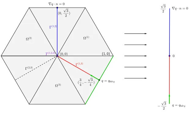
For some numerical simulations, the results of which are presented in Section 5, we pick the model in [15, 16] forM = 3phases with further choice of the mobility matrix (3.29). More precisely,wis of the form (3.13) with

wi,j(ϕ_ε) = 12

(ϕ(_εi))2(ϕ(_εj))2+ X k6=i,j

ϕ_ε(j)ϕ(_εk)(ϕ_ε(i))2+ϕ(_εi)ϕ(_εk)(ϕ_ε(j))2−ϕ(_εi)ϕ_ε(j)(ϕ(_εk))2

+ 4ΛX k6=i,j

(ϕ(_εi))2(ϕ_ε(j))2(ϕ(_εk))2, (3.35)

where the sixth order polynomial with a sufficiently largeΛ > 0 serves to prevent the leaking of third phase contributions between two other phases outside of the triple junction regions (see the discussion in Section 3.2). We choose a gradient potentialato be of the form (3.12) but independent ofϕ

εand define

ai,j(∇ϕ_ε) = 3 8

|∇ϕ(_εi)|2_+|∇ϕ(j)

ε |

2₋ X

k6=i,j

|∇ϕ(_εk)|2_{. (3.36)}

For the mobility matrixLin (3.29) we choose aqεdependent matrix defined as follows:

L(k,l)_(q

ε) =

(

−_3SkMc_(qεS¯₎(_Slqε₍)_qε), forl 6=k,

P

i6=l

McS¯(qε)

3Si(qε)Sl(qε), fork =l.

(3.37)

Here,Mc is a constant mobility parameter, Sk(qε) = ˜σi,k(qε) + ˜σj,k(qε)−σ˜i,j(qε) = −S˜(i,j,k)(qε)

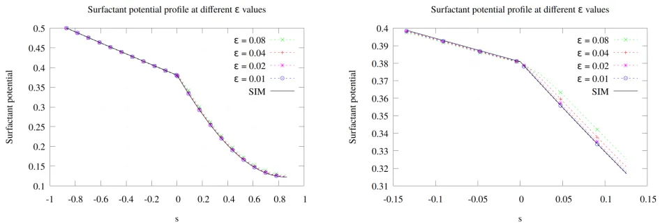
In the absence of fluid flow we obtain the following Cahn–Hilliard system: Fori= 1,2,3

∂tϕ(εi) =∇ ·

M_c

Si(qε)

∇µ(_εi), (3.38)

µ(_εi) =−3

4εSi(qε)∆ϕ

(i)

ε + 4 ¯S

ε Diw(qε, ϕε), (3.39)

where

Diw(qε, ϕ_ε) =

X

j6=i 1

Sj(qε)

∂_ϕ(i)

ε w(qε, ϕε)−∂ϕε(j)w(qε, ϕε)

.

4

Asymptotic Analysis

By matching suitable asymptotic expansions of solutions we show in this section that the formal asymptotic limit of the phase field model presented in Section 3.4 is the free boundary problem presented in Section 2.7. The situation in the phases and along the interface layers reduces to the two-phase case. Its asymptotic analysis is presented in [33] in great detail. We still present many details, for the notation is quite different under reformulation with multiple phase fields and, more importantly, we subsequently will require some of the findings to deal with the triple junctions. For the latter, techniques presented in [18, 19, 34] are used and further developed to treat the surfactant equation. The cased = 2, in which the triple junctions are points, is investigated first. Building on this, triple lines and quadruple points in the cased= 3are then considered.

4.1

Setting and assumptions

Let{ϕ

ε,jϕ,ε, µε,vε, pε, qε,jq,ε}ε>0denote a family of solutions to (3.28)–(3.34). We make some

as-sumptionson the model and the solutions, which are sketched here and further detailed and clarified

during the following analysis:

A1. We are interested in the solution regime where interfacial layers of thickness ∼ ε have

emerged between the domains in which the phase field is close to one of the minimisers of the multi-well potential w(qε, ϕ_ε). That is, these phases are where ϕ_ε ≈ ei for some

i∈ {1, . . . , M}and thus, notionally, the domain is occupied by fluidi.

A2. The potentials ai,j and wi,j are such that no third-phase contributions appear along the

in-terface layers. See Section 3.2 before (3.11) for a brief discussion and references. The clear meaning of this assumption and its consequences are discussed around equation (4.20) below.

A3. The potentials ai,j and wi,j furthermore are such that the equation forqε, (3.31) with (3.32),

A4. The mobilities of the phase fields are of the form

L(k,l)_(ϕ

ε, qε) =L

(k,l)

0 (ϕ_ε, qε) +εL

(k,l)

1 (ϕ_ε, qε),

where both the L(₀k,l) and the L(₁k,l) form symmetric matrices satisfying (3.20). Moreover,

L(k,l)_(e

j, qε) =0for allj ∈ {1, . . . , M}andqε∈Rbut ifϕˇ_ε∈ΣM\{ej}j then the kernel of

{L(₀k,l)(ˇϕ

ε, qε)}k,l is the span of1 = (1, . . . ,1)∈R

M_{. In turn, the matrix{L}(k,l)

1 (ϕ_ε, qε)}k,l is

non-degenerate for all(ϕ

ε, qε)∈Σ M _×

Rin the sense that its kernel is only the span of1.

4.2

Outer expansions and solutions

In points(x, t)in the phases away from the interface layers we consider expansions of the form

ζε(x, t) =ζ0(x, t) +εζ1(x, t) +ε2ζ2(x, t) +. . . ,

for all fields ϕ(εk), µ(εl), vε, pε, and qε, and also for the fluxes j(ϕ,εk). The flux jq,ε contains a term

scaling withε−1 _{whence we assume that it can be expanded in the form}

j_q,ε =ε−1jq,−1+ε0jq,0+. . . .

These expansions are plugged into the phase field equations (3.28)–(3.34) and all non-linearities are Taylor-expanded.

From (3.33) we obtain to leading order0that

∇ ·v0 = 0. (4.1)

Equation (3.30) yields to leading order−1that

0 = X i<j

˜

σi,j(q0)∂_ϕ(l)

ε wi,j(ϕ0)

for eachl = 1, . . . , M. As we are in a pure phase by assumption this implies thatϕ

0 is one of the

corners of the Gibb’s simplex,ϕ

0 = em for somem ∈ {1, . . . , M}. To the next order0we obtain

that

µ(₀l) =X m

X

i<j ˜

σi,j(q0)∂_ϕ(l) ε ϕ

(k)

ε wi,j(ϕ0)ϕ

(m)

1 , (4.2)

where we used thatξ_k0(ϕ(₀k)) = 0(thanks to (3.9)). Considering (3.28), (3.29) to leading order0yields

0 =−∇ ·j(_ϕ,k)₀, j(_ϕ,k)₀ =−X

l

L(₀k,l)(ϕ

0, q0)∇µ (l) 0 .

But asϕ

0 =emwe have thatL (k,l)

0 (ϕ₀, q0) = 0so that

Moreover,∂qL

(k,l)

0 (ϕ₀, q0) =0so that (3.28), (3.29) to the next order read

∂tϕ

(k)

1 +v0· ∇ϕ (k)

1 =−∇ ·j (k)

ϕ,1,

j(_ϕ,k)₁ =−X

l (∂ϕ

εL

(k,l)

0 (ϕ₀, q0)·ϕ₁+L1(k,l)(ϕ₀, q0))∇µ(0l).

Inserting (4.2) this becomes a parabolic problem forϕ

1that allows for the solutionϕ1 =0. Whether

this is the unique solution will depend on the boundary conditions both on the external boundary of the domain as well as the free boundaries. However, we do not need any specific knowledge of these solutions for our asymptotic analysis.

Aswi,j(ϕ₀) = 0there are no terms to order−1in the momentum equation (3.34). To order0it

yields that

∂t(ρ(m)v0) + (v0· ∇)(ρ(m)v0) = ∇ · −p0I+ 2η(m)D(v0)

, (4.4)

where we used that∂ϕ

εwi,j(ϕ0) = 0and (4.3).

Finally, recalling (3.17), using thatwi,j(ϕ₀) = 0and∂ϕ

εwi,j(ϕ0) = 0 in (3.32), and using (3.9)

we see that

j_q,−1 =−X

i<j

M_c(i,j)wi,j(ϕ₀)∇q0 =0, (4.5)

j_q,0 =− X

i

M_c(i)ξi(ϕ

(i)

0 )∇q0+

X

i<j

M_c(i,j) ∂ϕ_εwi,j(ϕ₀)·ϕ₁∇q0+wi,j(ϕ₀)∇q1

=−M_c(m)∇q0. (4.6)

The same arguments apply to the left-hand side of (3.31) so that, to order0, it reads

∂tc(m)(q0) +v0· ∇c(m)(q0) = −∇ ·jq,0 =∇ · M (m)

c ∇q0

.

With this equation and (4.1) and (4.4) we have recovered the bulk equations (2.39)–(2.41) of the sharp interface model.

4.3

Inner expansions and matching conditions

Consider now an interfacial layer between two domains whereϕ

0 ≈ enandϕ0 ≈ ep, respectively,

for two phase indicesn < p. For simplicity, we restrict the analysis to the two-dimensional case,

d= 2. However, the final results consisting of (4.31), (4.38), and (4.41) can also be retrieved in the higher dimensional case by following exactly the line of argument below. We refer to [64] for the techniques that are required to do so.

We use the limiting curve of the layer, which belongs to Γ(n,p)(t), in order to introduce new coordinates. Bys we denote a tangential coordinate along Γ(n,p)_{(t) such that, fort given, an}

∂sπ(n,p)(s, t)is a unit tangent vector field toΓ(n,p)(t). We assume the orientation ofsto be such that inx=π(n,p)_{(s, t)}

d dsτ

(n,p)_{(x, t) = κ}(n,p)_{(x, t) =:κ}(n,p)_{(x, t)ν}(n,p)_{(x, t), (4.7)}

where we introduced the scalar mean curvatureκ(n,p)_ofΓ(n,p)_{. Then}

d dsν

(n,p)_{(x, t) =−κ}(n,p)_{(x, t)τ}(n,p)_{(x, t).}

For any surface resident fieldr(t) : Γ(n,p)(t)→_R, written asR(s, t) =r(x, t),x=π(n,p)(s, t), in these new coordinates, we note the following identity (for instance, see [69] for a derivation):

∂tR(s, t)−∂tπ(n,p)(s, t)∂sR(s, t) = ∂ ◦(u(n,p)₎

t r(x, t), (4.8)

where we recall the notation (2.4) for the normal time derivative. A further coordinate in direction

ν(n,p)is denoted byz, which is the signed distance toΓ(n,p)(t)divided byε, i.e., positive on the side ofΩ(p)_{(t)and negative on the side ofΩ}(n)_(t).

As before, expansions of the solutions fields are plugged into the equations of the phase field model. But this time the expansions are of the form

ζε(x, t) = Z0(s, z, t) +εZ1(s, z, t) +ε2Z2(s, z, t) +. . . , (4.9a)

j(_ϕ,εk)(x, t) = ε−1J(_ϕ,−k)₁(s, z, t) +ε0J(_ϕ,k)₀(s, z, t) +ε1J(_ϕ,k)₁(s, z, t) +. . . , (4.9b)

j_q,ε(x, t) = ε−2Jq,−2(s, z, t) +ε−1Jq,−1(s, z, t) +ε0Jq,0(s, z, t) +. . . , (4.9c)

for inner variablesZ ∈ {Φ_ε,M_ε, Qε,Vε, Pε}corresponding to{ϕ_ε, µ_ε, qε,vε, pε}in points(x, t)

close toΓ(n,p)(t)where the distance function, which is required to define the coordinatez, is well-defined. The tangential coordinatesfor such a pointxis such thatπ(n,p)_{(s, t)is the closest point to}

xonΓ(n,p)_{. The differential operators read as follows in the new coordinates [33]:}

∂tζ(x, t) =−ε−1u(n,p)∂zZ(s, z, t) +∂tZ(s, z, t)−∂tπ(n,p)∂sZ(s, z, t) +O(ε), (4.10a)

∇ζ(x, t) =ε−1∂zZ(s, z, t)ν(n,p)+ (1 +εκ(n,p))∂sZ(s, z, t)τ(n,p)+O(ε2). (4.10b)

Here and in the following all interface resident fields such asu(n,p),ν(n,p), andτ(n,p)are evaluated inπ(n,p)_{(s, t)∈Γ}(n,p)_(t).

Requiring inner and outer expansions to match leads to the followingmatching conditions[36]:

Asz → ±∞,

Z0(s, z, t)∼ζ0±, (4.11)

∂zZ0(s, z, t)∼0, (4.12)

∂zZ1(s, z, t)∼ ∇ζ0±·ν

J(_ϕ,−k)₁(s, z, t)∼0, Jq,−2(s, z, t)∼0, (4.14)

J_ϕ,(k)₀(s, z, t)∼(j_ϕ,(k₀))±, Jq,−1(s, z, t)∼j±q,−1, (4.15)

J_ϕ,(k)₁(s, z, t)∼(j(_ϕ,k)₁)±+z∇(j_ϕ,(k)₀)±ν(n,p), Jq,0(s, z, t)∼j±q,0+z∇j

± q,−1ν

(n,p)_,

(4.16)

where(·)±denotes the limitlimδ&0(·)(x±δν(n,p))inx=π(n,p)(s, t)∈Γ(n,p)(t).

4.4

Inner solutions

The surfactant equation (3.31), (3.32) to leading order−3reads

0 =−ν(n,p)·∂zJq,−2,

Jq,−2 =−

X

i<j

M_c(i,j) ai,j(Φ0, ∂zΦ0⊗ν(n,p)) +wi,j(Φ0)

∂zQ0ν(n,p). (4.17)

Integrating with respect to z from −∞ to a variable denoted by z again and using the matching

condition (4.14) we conclude that∂zQ0 = 0so that also all fields depending onQ0such asσ˜i,j(Q0)

are constant across the interface layer to leading order. In particular,

q0

p

n= 0, q0 ±

(π(n,p)(s, t), t) = Q0(s, t) (4.18)

thanks to the matching condition (4.11). Equation (3.30) to order−1then becomes

0 =X i<j

˜

σi,j(Q0)

−ν(n,p)· d

dz ∂∇ϕ(εl)ai,j(Φ0, ∂zΦ0⊗ν

(n,p)₎

+∂_ϕ(l)

ε ai,j(Φ0, ∂zΦ0 ⊗ν

(n,p)

) +∂_ϕ(l)

ε wi,j(Φ0)

. (4.19) This second order ODE inz is supplied with the boundary conditionsΦ₀ ∼ e_p, e_n and∂zΦ0 ∼ 0

asz → ±∞, which are due to the matching conditions (4.11), (4.12). By Assumption A2 on the

potentialsai,j andwi,j there are no third phase contributions, i.e., the leading order solution Φ0 is

such thatΦ(₀k) = 0ifk 6∈ {p, n}. In fact, with choices as in [15, 37, 70], for a wide range of surface energiesγi,j and related tensionsσ˜i,jthe solution only depends onz and is of the form

Φ₀(z) = χ(z)e_p+ (1−χ(z))e_n, (4.20)

with some monotone functionχ:_R→[0,1](thetransition profile) satisfying

χ(0) = 1

2, z→∞lim χ(z) = 1, z→−∞lim χ(z) = 0.

The potentials are also such that for i < j then ai,j(Φ0, ∂zΦ0 ⊗ν(n,p)) = 0 and wi,j(Φ0) = 0 if

(i, j)6= (n, p). Hence,Φ₀ satisfies

0 = ˜σn,p(Q0)

∂_ϕ(l)

ε an,p(Φ0, ∂zΦ0⊗ν

(n,p)_{) +∂}

ϕ(εl)wn,p(Φ0)

− d

dz ∂∇ϕ(εl)an,p(Φ0, ∂zΦ0⊗ν

(n,p)₎