warwick.ac.uk/lib-publications
Manuscript version: Author’s Accepted Manuscript
The version presented in WRAP is the author’s accepted manuscript and may differ from the
published version or Version of Record.
Persistent WRAP URL:
http://wrap.warwick.ac.uk/91792
How to cite:
Please refer to published version for the most recent bibliographic citation information.
If a published version is known of, the repository item page linked to above, will contain
details on accessing it.
Copyright and reuse:
The Warwick Research Archive Portal (WRAP) makes this work by researchers of the
University of Warwick available open access under the following conditions.
Copyright © and all moral rights to the version of the paper presented here belong to the
individual author(s) and/or other copyright owners. To the extent reasonable and
practicable the material made available in WRAP has been checked for eligibility before
being made available.
Copies of full items can be used for personal research or study, educational, or not-for-profit
purposes without prior permission or charge. Provided that the authors, title and full
bibliographic details are credited, a hyperlink and/or URL is given for the original metadata
page and the content is not changed in any way.
Publisher’s statement:
Please refer to the repository item page, publisher’s statement section, for further
information.
Multi-locus data distinguishes between population growth and
multiple merger coalescents
Jere Koskela
j.koskela@warwick.ac.uk
Department of Statistics
University of Warwick
Coventry, CV4 7AL
United Kingdom
April 19, 2018
Abstract
We introduce a low dimensional function of the site frequency spectrum that is
tailor-made for distinguishing coalescent models with multiple mergers from Kingman coalescent
models with population growth, and use this function to construct a hypothesis test between
these model classes. The null and alternative sampling distributions of the statistic are
intractable, but its low dimensionality renders them amenable to Monte Carlo estimation.
We construct kernel density estimates of the sampling distributions based on simulated data,
and show that the resulting hypothesis test dramatically improves on the statistical power
of a current state-of-the-art method. A key reason for this improvement is the use of
multi-locus data, in particular averaging observed site frequency spectra across unlinked loci to
reduce sampling variance. We also demonstrate the robustness of our method to nuisance
and tuning parameters. Finally we show that the same kernel density estimates can be used
to conduct parameter estimation, and argue that our method is readily generalisable for
applications in model selection, parameter inference and experimental design.
1
Introduction
The Kingman coalescent [Kingman, 1982a,b,c, Hudson, 1983a,b, Tajima, 1983] describes the
random ancestral relations among DNA sequences sampled from large populations, and is a
prominent model with which to make predictions about genetic diversity. This popularity derives
from its robustness: a wide class of genealogical models all have the Kingman coalescent, or a
variant of it, as their limiting process when the population size is large [M¨
ohle, 1998]. Together,
the Kingman coalescent and the infinitely-many-sites (IMS) model also form a tractable model
of genetic evolution [Watterson, 1975]. Hence, many inference methods based on the Kingman
coalescent have been developed; see e.g. Donnelly and Tavar´
e [1995], Hudson [1990], Nordborg
[2001], Hein et al. [2005] or Wakeley [2007] for reviews.
The site frequency spectrum (SFS) at a given locus is an important and popular statistic by
which to summarise genetic data under the IMS model and a coalescent process. Quantities of
interest, such as the expectations and covariances of the SFS, are easily computed under the
Kingman coalescent [Fu, 1995].
Despite its robustness, many evolutionary histories can also lead to significant deviations from
the Kingman coalescent. A variety of statistical tools is available for detecting such deviations,
e.g. Tajima’s
D
[Tajima, 1989], Fu and Li’s
D
[Fu and Li, 1993] or Fay and Wu’s
H
[Fay and Wu,
of the actual evolutionary mechanisms leading to the deviation from the Kingman coalescent.
Eldon et al. [2015] investigated the ability of a single-locus SFS to distinguish two different
deviations from the Kingman coalescent:
1. population growth, in particular exponential or algebraic population growth, and
2. gene genealogies described by so-called Λ-coalescents [Sagitov, 1999, Pitman, 1999,
Don-nelly and Kurtz, 1999] featuring multiple mergers. There is growing evidence that such
coalescents are an appropriate model for organisms with high fecundity coupled with
a skewed offspring distribution [Beckenbach, 1994, ´
Arnason, 2004, Eldon and Wakeley,
2006, Sargsyan and Wakeley, 2008, Hedgecock and Pudovkin, 2011, Birkner et al., 2011,
Steinr¨
ucken et al., 2013, Tellier and Lemaire, 2014].
Both scenarios lead to an excess of singletons in the SFS compared to the Kingman coalescent,
leading e.g. to a negative value of Tajima’s
D
[Durrett and Schweinsberg, 2005]. Eldon et al.
[2015] showed that a single-locus SFS can distinguish between scenarios 1 and 2 with moderate
statistical power, at least when the rate of mutation was sufficiently high and the deviation from
the Kingman coalescent, the population growth rate in the scenario 1 and the prevalence of
multiple mergers in scenario 2, was sufficiently large.
The present work builds on the result of Eldon et al. [2015] by proposing a new statistical test to
distinguish between scenarios 1 and 2. A key development is that the proposed tests are based
on multiple site frequency spectra corresponding to multiple unlinked loci. Modern sequencing
technologies have made sequence data from multiple linkage groups commonplace, and we show
that making use of multi-locus data in this way greatly improves the power of statistical tests.
We assume that no recombination takes place within loci.
In addition, we extend the work of Eldon et al. [2015] by explicitly including diploidy into
the models under consideration. Specifically, we consider a diploid, biparental population with
symmetric mating, and with each parent contributing a single chromosome to their offspring.
This results in ancestries modeled as time-changed Kingman coalescents in scenario 1, and
Ξ-coalescents, incorporating up to four simultaneous mergers of groups of multiple lineages, in
scenario 2 [Birkner et al., 2013a]. In brief, the presence of up to four simultaneous mergers arises
because genetic material at given locus can coalesce at either copy in either diploid parent.
While our new statistical tests contain the population rescaled mutation rate,
θ/
2, as a nuisance
parameter, we show empirically that the statistical power achieved by our method is extremely
robust to misspecification of this parameter. Hence, in practice relying on a generalised
Wat-terson estimator for the mutation rate can be expected to produce reliable inferences.
In addition to selecting the model class which best explains the data, it is also of interest to infer
those parameters within that class which result in the best fit. Hence, parameter inference for
Λ- and Ξ-coalescents has been a growing area of research in recent years [Eldon and Wakeley,
2006, Birkner and Blath, 2008, Sargsyan and Wakeley, 2008, Eldon and Wakeley, 2009, Birkner
et al., 2011, Eldon, 2011, Birkner et al., 2013b, Steinr¨
ucken et al., 2013, Koskela et al., 2015,
2
Summary statistic and approximate likelihood
Consider a sample of
n
DNA sequences taken at a given genetic locus, and assume that derived
mutations can be distinguished from ancestral states. For
n
∈
N
let [
n
] :=
{
1
, . . . , n}
, and let
ξ
i
(
n
)
denote the total number of sites at which the mutant base appears
i
∈
[
n
−
1] times. Then
ξ
(
n
)
:=
ξ
1
(
n
)
, . . . , ξ
n
(
n
−
)
1
is referred to as the
unfolded
site-frequency spectrum based on the
n
DNA sequences. If mutant
and ancestral type cannot be distinguished, the
folded
spectrum
η
(
n
)
:= (
η
1
(
n
)
, . . . , η
(
b
n
n/
)
2
c
) [Fu,
1995] is often considered instead, where
η
(
i
n
)
:=
ξ
(
n
)
i
+
ξ
(
n
)
n
−
i
1 +
δ
i,n
−
i
,
1
≤
i
≤ bn/
2
c,
and
δ
i,j
= 1 if
i
=
j
, and is zero otherwise. Define
ζ
(
n
)
=
ζ
1
(
n
)
, . . . , ζ
n
(
n
−
)
1
as the normalised
unfolded SFS, whose entries are given by
ζ
i
(
n
)
:=
ξ
i
(
n
)
/|ξ
(
n
)
|
, where
|ξ
(
n
)
|
:=
ξ
(
n
)
1
+
· · ·
+
ξ
(
n
)
n
−
1
is
the total number of segregating sites. We adopt the convention that
ζ
(
n
)
=
0
if there are no
segregating sites.
Even though both scenarios 1 and 2 predict an excess of singletons, Eldon et al. [2015] showed
that the expected tail of the normalised SFS varies between the two when the singletons have
been matched [Eldon et al., 2015, Figure 1]. Hence we define the lumped tail
ζ
(
k
n
)
:=
n
−
1
X
j
=
k
ζ
j
(
n
)
,
3
≤
k
≤
n
−
1
(1)
and consider the summary statistic (
ζ
1
(
n
)
, ζ
(
k
n
)
) for some fixed
k
, to be specified. This
two-dimensional summary of the SFS can be expected to distinguish scenarios 1 and 2, while
ex-ploiting a lower dimensionality to reduce sampling variance (see the discussion on the effect
of lumping in [Eldon et al., 2015] for an account of the same phenomenon in the context of
approximate Bayesian computation) and reduce the number of Monte Carlo simulations needed
to robustly characterise its sampling distribution.
We make use of multi-locus data by computing an SFS independently for each locus, and
av-eraging over all available loci to reduce variance. To this end, let (
ζ
1
(
n
)
(
j
)
, ζ
(
k
n
)
(
j
)) denote the
singleton class and lumped tail corresponding to the
j
th
locus, and
(
ζ
1
(
n
,L
)
, ζ
(
k,L
n
)
) :=
1
L
L
X
j
=1
(
ζ
1
(
n
)
(
j
)
, ζ
(
k
n
)
(
j
))
(2)
denote the mean singletons and lumped tail when there are
L
loci. A description of how (2) can
be computed from observed data, as well as from simulated trees, is provided in the appendix.
Remark 1.
In scenario 1, and for binary, Kingman-type coalescents in general, (2) converges
to its expected value as
L
→ ∞
due to the strong law of large numbers.
In contrast, in
scenario 2, and for multiple merger coalescents in general, unlinked loci have positively correlated
coalescence times and hence a law of large numbers does not hold. This is easily verified by
considering a haploid sample of size 2 from 2 unlinked loci. Let
λ
n,k
:= Λ(
{
0
}
)
1
{
k
=2
}
+
Z
(0
,
1]
be the usual merger rate of any 2
≤
k
≤
n
lineages under a Λ-coalescent.
Let
T
i
be the
coalescence time at locus
i
∈ {
1
,
2
}
. Note that
E
[
T
i
] = 1, and that the total rate of effective
mergers among the four lineages is
2
λ
4
,
2
+ 4
λ
4
,
3
+
λ
4
,
4
.
By conditioning on whether the first merger involves four lineages (an event of probability
λ
4
,
4
/
(2
λ
4
,
2
+ 4
λ
4
,
3
+
λ
4
,
4
)) or strictly fewer than four lineages (an event of the complementary
probability), it is straightforward to verify that
E
[
T
1
T
2
] =
1
2
λ
4
,
2
+ 4
λ
4
,
3
+
λ
4
,
4
1 +
2
−
λ
4
,
4
2
λ
4
,
2
+ 4
λ
4
,
3
+
λ
4
,
4
=
1
2
−
λ
4
,
4
1 +
2
−
λ
4
,
4
2
−
λ
4
,
4
=
2
2
−
λ
4
,
4
>
1 whenever Λ
6
=
δ
0
,
where the second line follows from the expansions
λ
4
,
3
=
λ
3
,
3
−
λ
4
,
4
,
λ
4
,
2
= 1
−
2
λ
3
,
3
+
λ
4
,
4
.
Hence,
Cov(
T
1
, T
2
) = 0
⇔
Λ =
δ
0
,
and a slightly more cumbersome version of this calculation verifies the same statement for
Ξ-coalescents. Sampling variance will still be reduced by averaging across unlinked loci, but by
less than in scenario 1, and an
L
→ ∞
limit will be random if it exists.
Let Π denote an arbitrary coalescent process,
θ/
2 denote a population-rescaled mutation rate,
and
P
Π
,θ
(
ζ
1
(
,L
n
)
, ζ
(
k,L
n
)
) denote the sampling distribution of (2) under the coalescent Π and mutation
rate
θ/
2. This distribution is intractable, but if it were available then the likelihood ratio test
statistic
sup
Π
∈
Θ
1,θ>
0
P
Π
,θ
(
ζ
(
n
)
1
,L
, ζ
(
n
)
k,L
)
sup
Π
∈
Θ
0,θ>
0
P
Π
,θ
(
ζ
(
n
)
1
,L
, ζ
(
n
)
k,L
)
(3)
would be a desirable tool for distinguishing between coalescent models in the class Θ
0
, the null
hypothesis, from an alternative class Θ
1
, based on an observed value of (2).
Eldon et al. [2015] proposed a Poisson approximation to a test akin to (3), based on the whole
unnormalised SFS, by assuming that the hidden coalescent ancestry of their sample coincided
with the expected coalescent branch lengths. These expected branch lengths were then computed
by recursion. The number of mutations was also assumed to always coincide exactly with the
number of observed segregating sites, in what is known as the “fixed-
s
” method [see e.g. Depaulis
and Veuille, 1998, Ramos-Onsins and Rozas, 2002]. In this paper we approximate
P
Π
,θ
by
simulation directly. This avoids the unquantifiable bias introduced by the Poisson and fixed-
s
approximations, and is scalable because only a two-dimensional sampling distribution needs to
be approximated, regardless of the sample size or the number of alleles. Of course replacing
the sampling distributions in (3) with estimators will itself introduce bias, but provided that
the estimators are close to the truth then it is reasonable to expect the bias to be small in
comparison to an ad-hoc Poisson approximation. In particular, Figure 12 in Section 4 shows no
evidence of bias when using our approximate sampling distributions to infer parameters.
In order to produce an approximate sampling distribution ˆ
P
Π
,θ
, a simulation algorithm was
developed for producing samples from a specified coalescent Π with mutation rate
θ/
2. The
algorithm takes as inputs a sample size and a desired number of unlinked loci per sample,
within which we assume no recombination takes place. The method is described in detail in the
appendix, and a C++ implementation is available at
https://github.com/JereKoskela/Beta-Xi-Sim. Three diploid model classes have been implemented:
1. Beta(2
−
α, α
)-Ξ-coalescents for
α
∈
[1
,
2] derived from Λ-coalescents with Λ = Beta(2
−
α, α
) by randomly splitting all merging lineages into four groups, and coalescing each group
separately as in [Birkner et al., 2013a, equation (29)] and [Blath et al., 2016, equation (15)],
2. the Kingman coalescent with exponential population growth at rate
γ >
0,
3. the Kingman coalescent with algebraic population growth with exponent
γ >
0.
Implementations for further model classes, such as Ξ-coalescents driven by measures other than
the Beta(2
−
α, α
) class or derived from more general models of mating patterns, such as those
described in [Birkner et al., 2017], could be easily added. Further evolutionary forces such as
natural selection could also be incorporated, though naturally both of these generalisation come
at increased computational cost.
Once a sample of simulated realisations of (2) has been produced under the desired null and
alternative hypotheses (or suitable discretisations in the case of interval hypotheses), kernel
density estimators were fitted to these samples using the
kde
function in the
ks
package
(ver-sion 1.10.4) in
R
under default settings. For a comprehensive introduction to kernel density
estimation, see e.g. [Scott, 1992]. In particular, the bandwitdh is determined using the SAMSE
estimator of [Duong and Hazelton, 2003, equation (6)] as implemented in the
Hpi
function of the
aforementioned
ks
package. This package allows kernel density estimation in up to six
dimen-sions, so that higher dimensional statistics could be used to distinguish model classes that are
not well separated by just singletons and the lumped tail. However, this increase in
dimensional-ity would come at the cost of increasingly intensive simulation time as more samples are needed
to accurately represent a higher dimensional sampling distribution, and was not necessary for
our purposes.
Once these kernel density estimators have been produced, they can be substituted into (3) to
obtain an approximation
sup
Π
∈
Θ
1
,θ>
0
P
ˆ
Π
,θ
(
ζ
(
n
)
1
,L
, ζ
(
n
)
k,L
)
sup
Π
∈
Θ
0
,θ>
0
P
ˆ
Π
,θ
(
ζ
(
n
)
1
,L
, ζ
(
n
)
k,L
)
.
However, simulating samples and producing kernel density estimators for combinations of
coa-lescent processes and mutation rates also incurs a significant computational cost. To alleviate it,
we assume that a computationally cheap estimator ˆ
θ
is available, e.g. the generalised Watterson
estimator
ˆ
θ
=
|ξ
(
n
)
|/
E
Π
[
T
(
n
)
]
,
where
E
Π
[
T
(
n
)
] denotes the expected tree length from
n
leaves under coalescent mechanism Π.
We then consider the test statistic
sup
Π
∈
Θ
1
P
ˆ
Π
,
θ
ˆ
(
ζ
(
n
)
1
,L
, ζ
(
n
)
k,L
)
sup
Π
∈
Θ
0
P
ˆ
Π
,
θ
ˆ
(
ζ
(
n
)
1
,L
, ζ
(
n
)
k,L
)
(4)
The statistic (4) is straightforward to evaluate pointwise, and further simulated data can be
used to obtain an empirical quantile
ρ
ε
such that
sup
Π
∈
Θ
0
P
Π
,
θ
ˆ
sup
Π
∈
Θ
1
P
ˆ
Π
,
θ
ˆ
(
ζ
(
n
)
1
,L
, ζ
(
n
)
k,L
)
sup
Π
∈
Θ
0
P
ˆ
Π
,
θ
ˆ
(
ζ
(
n
)
1
,L
, ζ
(
n
)
k,L
)
≥
ρ
ε
≤
ε,
where
P
Π
,
θ
ˆ
denotes the law of the coalescent process under coalescent mechanism Π and mutation
rate ˆ
θ/
2. Given such a quantile, a hypothesis test of approximate size
ε
for an observed pair
(
ζ
1
(
n
,L
)
, ζ
(
k,L
n
)
) is given by
Φ(
ζ
1
(
n
,L
)
, ζ
(
k,L
n
)
) =
0
if
sup
Π
∈
Θ1
P
ˆ
Π
,
ˆ
θ
(
ζ
(
n
)
1
,L
,ζ
(
n
)
k,L
)
sup
Π
∈
Θ0
P
ˆ
Π
,
θ
ˆ
(
ζ
(
n
)
1
,L
,ζ
(
n
)
k,L
)
≤
ρ
ε
1
if
sup
Π
∈
Θ1
P
ˆ
Π
,
ˆ
θ
(
ζ
(
n
)
1
,L
,ζ
(
n
)
k,L
)
sup
Π
∈
Θ0
P
ˆ
Π
,
θ
ˆ
(
ζ
(
n
)
1
,L
,ζ
(
n
)
k,L
)
> ρ
ε
,
(5)
where Φ(
ζ
1
(
n
,L
)
, ζ
(
k,L
n
)
) = 1 corresponds to rejecting the null hypothesis. The size of the test is only
approximate because the quantile
ρ
ε
is computed from finitely many simulated realisations, and
because the sampling distribution ˆ
P
Π
,
θ
ˆ
is itself a kernel density approximation. In the next
section we demonstrate the performance and robustness of this test, and compare it to the
Poisson-fixed-
s
test of Eldon et al. [2015].
Remark 3.
Hypothesis tests only provide information on the model fit of the alternative
hy-pothesis relative to the null. Hence, if the null hyhy-pothesis is a poor fit to the data, a high value
of (4) does not necessarily indicate that the alternative hypothesis is a good fit, but only a
better one than the null hypothesis. The empirical sampling distributions constructed in order
to evaluate (4) can be used to address this ambiguity to some extent, e.g. by plotting observed
data along with simulated realisations in scatter plots akin to Figure 1 in the next section. This
ability to overcome a limitation of hypothesis tests arises out of the low dimensionality of the
statistic (2), and the ease with which its sampling distribution can hence be visualised.
3
Results: model selection
In this section we present simulation studies demonstrating the statistical power and robustness
of (5). For comparison, the same simulation study will also be undertaken using the
Poisson-fixed-
s
approximate likelihood ratio test of [Eldon et al., 2015]. For ease of computation we
discretise the null and alternative hypotheses, and take them to be
Θ
0
:=
{
Kingman coalescent with exponential or algebraic growth, each at rates
γ
∈ {
0
,
0
.
1
,
0
.
2
, . . . ,
0
.
9
,
1
,
1
.
5
,
2
,
2
.
5
,
3
,
3
.
5
,
4
,
5
,
6
, . . . ,
19
,
20
,
25
,
30
,
35
,
40
,
50
,
60
, . . . ,
990
,
1000
}},
Θ
1
:=
{
Beta(2
−
α, α
)-Ξ-coalescents with
α
∈ {
1
,
1
.
025
, . . . ,
1
.
975
,
2
}},
respectively. The somewhat irregular discretisation has been chosen to yield comprehensive
coverage of the sampling distribution of the continuous hypotheses based on trial runs (see
Figure 1). Note that all three model classes coincide with the Kingman coalescent at the far
left end of the cloud of points, which corresponds to
γ
= 0 in scenario 1 and
α
= 2 in scenario
2. We also fix the approximate sizes of all hypothesis tests at
ε
= 0
.
01.
0.0
0.2
0.4
0.6
0.8
1.0
0.0
0.2
0.4
0.6
0.8
1.0
n = 100; k = 15; L = 23
Normalised singletons
Nor
malised 15+ lumped tail
0.0
0.2
0.4
0.6
0.8
1.0
0.0
0.2
0.4
0.6
0.8
1.0
n = 500; k = 15; L = 23
Normalised singletons
Nor
[image:8.595.75.511.82.289.2]malised 15+ lumped tail
Figure 1: Scatter plot of the joint distribution of the summary statistic (2) with
L
= 23 loci,
lumping from
k
= 15 and sample size
n
= 100 on the left and
n
= 500 on the right. Red
dots denote realisations from a Beta(2
−α, α
)-Ξ-coalescent, green dots from an algebraic growth
coalescent, and blue dots from an exponential growth coalescent. The runtimes to generate these
samples on a single Intel i5-2520M 2.5 GHz processor were 6.5 hours for
n
= 100, and 59 hours
for
n
= 500.
Beta(2
−
α, α
)-Ξ-coalescent from a class of binary coalescents is harder than distinguishing the
corresponding Beta(2
−
α
)-Λ-coalescent from the same binary class. This is because randomly
assigning mergers into four groups can splits multiple mergers into either outright binary
merg-ers, or smaller multiple mergers. Thus, the SFS of the resulting Ξ-coalescent tree will resemble
the SFS of a binary coalescent more closely than the same Λ-coalescent tree would have done.
For each of the coalescent processes in Θ
0
and Θ
1
, we simulated 1000 replicates of samples
of size
n
= 100 and
n
= 500, with
L
= 23 unlinked loci and with per-locus mutation rates
θ
i
/
2 =
N
e
α
−
1
L
i
µ
, with effective population size
N
e
= 1000, per-site-per-generation mutation rate
set at either
µ
= 10
−
8
or 10
−
7
, and the number of sites per locus varying between
L
i
= 19
×
10
6
and
L
i
= 31
×
10
6
as recorded for the linkage groups of Atlantic cod in [Tørresen et al., 2017,
Supplementary Table 3]. Atlantic cod is a species for which multiple mergers have frequently
been suggested as an important evolutionary mechanism [see e.g. Steinr¨
ucken et al., 2013, Tellier
and Lemaire, 2014, and references therein]. The scaling parameter
α
in the mutation rate denotes
the parameter of the Θ
1
class, with
α
= 2 corresponding to the Kingman coalescent as per the
scaling results of Schweinsberg [2003]. For each coalescent, the 1000 replicates were split into
two groups: 500 replicates as training data for computing the kernel density estimator ˆ
P
Π
,
θ
ˆ
,
and an independent 500 replicates as test data from which to estimate the empirical size and
power of the hypothesis test (5).
We also simulated independent realisations of the “fixed-
s
” data sets of Eldon et al. [2015]
to facilitate a comparison, keeping the total number of segregating sites at
s
= 50 as in the
original article. We extend their Poisson-fixed-
s
approximate likelihood test to our multi-locus
setting in two ways: by treating multiple loci as independent, or averaging over them as in the
KDE case. Furthermore, we approximate the expected branch lengths required by the “fixed-
s
”
method by averaging over 100 000 coalescent simulations, in contrast with the exact, numerical
computations carried out by Eldon et al. [2015]. This makes our “fixed-
s
” results slightly noisier,
While solvable recursions for Ξ-coalescent expected branch lengths are known [Blath et al., 2016],
they are much more computationally intensive than their Λ-coalescent counterparts. Moreover,
the exact branch length approach cannot be easily extended to cover more complex scenarios,
which are nevertheless easy to simulate. A comparison of the empirical power as a function of
the
α
-parameter in the Beta(2
−
α, α
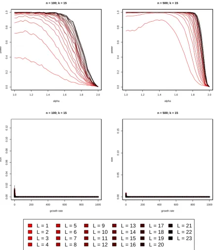
)-distribution is presented in Figure 2.
● ● ● ● ● ● ● ●
● ●
● ● ● ●
● ● ● ● ● ●
● ●
● ●
●
● ● ●
●
● ●
● ●
● ●
● ●
● ●
● ●
1.0
1.2
1.4
1.6
1.8
2.0
0.0
0.2
0.4
0.6
0.8
1.0
n = 100; k = 15; L = 23; s = 50
alpha
po
w
er
x
x x
x
x x
x
x x
x
x x
x x x
x x
x x x x
x x x x x x x
x x x x x x x x x x x x x
1.0
1.2
1.4
1.6
1.8
2.0
0.0
0.2
0.4
0.6
0.8
1.0
+ + + + + + + + + + + + + + + + + + + + + + + + +
+ +
+
+
+
+
+
+
+
+
+
+
+
+
+ +
1.0
1.2
1.4
1.6
1.8
2.0
0.0
0.2
0.4
0.6
0.8
1.0
* *
*
* *
* *
*
* *
*
* * * *
*
* * *
*
*
* *
* *
* *
* * *
* * * * *
* * * * * *
1.0
1.2
1.4
1.6
1.8
2.0
0.0
0.2
0.4
0.6
0.8
1.0
+
*
o
x
Averaged KDE
KDE
Averaged fixed s
Fixed s
● ● ● ● ● ● ● ● ● ● ● ● ● ● ● ● ● ● ● ● ● ● ● ● ● ●
● ● ● ●
● ●
●
●
● ●
●
●
● ●
●
1.0
1.2
1.4
1.6
1.8
2.0
0.0
0.2
0.4
0.6
0.8
1.0
n = 500; k = 15; L = 23; s = 50
alpha
po
w
er
x x x x x x x x
x x x
x x
x x
x
x
x x
x
x
x
x x
x
x
x
x
x
x
x
x x
x
x x x x x
x x
1.0
1.2
1.4
1.6
1.8
2.0
0.0
0.2
0.4
0.6
0.8
1.0
+ + + + + + + + + + + + + + + + + + + + + + + + + + + + + + + + + +
+
+
+
+
+
+
+
1.0
1.2
1.4
1.6
1.8
2.0
0.0
0.2
0.4
0.6
0.8
1.0
* * *
* * * *
* *
* * *
* *
* *
* * * *
*
*
*
*
*
*
*
*
*
*
*
*
*
*
*
*
*
* * * *
1.0
1.2
1.4
1.6
1.8
2.0
0.0
0.2
0.4
0.6
0.8
1.0
+
*
o
x
Averaged KDE
KDE
Averaged fixed s
Fixed s
●
●
● ● ● ●
●●●●●●●●●●●●●●●●●●●●●●●●●●●●●●●●●●●●●●●●●●●●●●●●●●●●●●●●●●●●●●●●●●●●●●●●●●●●●●●●●●●●●●●●●●●●●●●●●●●●●●●●●●●●●●●●●●●●●●●●●●●●●●●
0
200
400
600
800
1000
0.000
0.005
0.010
0.015
0.020
n = 100; k = 15; L = 23; s = 50
growth rate
siz
e
x
x
x
x
x
x
x
x
x
x
x
x
x
x
x
x
x
x
x
x
x
x
x
x
x
x
x
x
x
x
x
x
xxxxxxxxxxxxxxxxxxxxxxxxxxxxxxxxxxxxxxxxxxxxxxxxxxxxxxxxxxxxxxxxxxxxxxxxxxxxxxxxxxxxxxxxxxxxxxxxxxxxx
0
200
400
600
800
1000
0.000
0.005
0.010
0.015
0.020
+
+
+
+
+
+
+
+
+
+
+
+
+
+
+
+
+
+
+
+
+
+
+
+
+
+
+
+
+
+
+
+
+++++++++++++++++++++++++++++++++++++++++++++++++++++++++++++++++++++++++++++++++++++++++++++++++++++
0
200
400
600
800
1000
0.000
0.005
0.010
0.015
0.020
*
*
*
*
**
*
*
*
**
**************************************************************************************************************************
0
200
400
600
800
1000
0.000
0.005
0.010
0.015
0.020
●
● ●
●
●
● ● ● ● ●
● ● ● ● ● ●
●●●●●●●●●●●●●●●●●●●●●●●●●●●●●●●●●●●●●●●●●●●●●●●●●●●●●●●●●●●●●●●●●●●●●●●●●●●●●●●●●●●●●●●●●●●●●●●●●●●●●●●●●●●●●●●●●●●●●
0
200
400
600
800
1000
0.000
0.005
0.010
0.015
0.020
x
x
x
x
x
x
x
x
x
x
x
x
x
x
x
x
x
x
x
x
x
x
x
x
x
x
x
x
x
x
x
x
xxxxxxxxxxxxxxxxxxxxxxxxxxxxxxxxxxxxxxxxxxxxxxxxxxxxxxxxxxxxxxxxxxxxxxxxxxxxxxxxxxxxxxxxxxxxxxxxxxxxx
0
200
400
600
800
1000
0.000
0.005
0.010
0.015
0.020
+
+
+
+
+
+
+
+
+
+
+
+
+
+
+
+
+
+
+
+
+
+
+
+
+
+
+
+
+
+
+
+
+++++++++++++++++++++++++++++++++++++++++++++++++++++++++++++++++++++++++++++++++++++++++++++++++++++
0
200
400
600
800
1000
0.000
0.005
0.010
0.015
0.020
*
*
*
*
**
*
*
*
**
**************************************************************************************************************************
0
200
400
600
800
1000
0.000
0.005
0.010
0.015
0.020
+
*
o
x
Averaged KDE
KDE
Averaged fixed s
Fixed s
●
● ● ●
● ● ● ● ● ●
●●●●●●●●●●●●●●●●●●●●●●●●●●●●●●●●●●●●●●●●●●●●●●●●●●●●●●●●●●●●●●●●●●●●●●●●●●●●●●●●●●●●●●●●●●●●●●●●●●●●●●●●●●●●●●●●●●●●●●●●●●●
0
200
400
600
800
1000
0.000
0.005
0.010
0.015
0.020
n = 500; k = 15; L = 23; s = 50
growth rate
siz
e
x
x
x
x
x
x
x
x
x
x
x
x
x
x
x
x
x
x
x
x
x
x
x
x
x
x
x
x
x
x
x
x
xx
xxxxxxxxxxx
x
xx
xx
x
xx
xx
x
xx
x
xx
xxx
xx
xxxx
xxx
xxx
x
x
x
xxxxxxxx
x
xx
xx
x
xx
x
x
xxxxxxx
xxx
x
xxxxxxx
x
x
xxxxxxxxxxxxxxxx
0
200
400
600
800
1000
0.000
0.005
0.010
0.015
0.020
+
+
+
+
+
+
+
+
+
+
+
+
+
+
+
+
+
+
+
+
+
+
+
+
+
+
+
+
+
+
+
+
+++++++++++++++++++++++++++++++++++++++++++++++++++++++++++++++++++++++++++++++++++++++++++++++++++++
0
200
400
600
800
1000
0.000
0.005
0.010
0.015
0.020
*
***
**
*
***
**
*
*
*
**
*
*
*******
*
*
*******************************************************************************
**
*
******
*
**
***
*
***
*
****
*
*
0
200
400
600
800
1000
0.000
0.005
0.010
0.015
0.020
●
● ●
●
● ● ●
● ● ● ●
● ● ● ● ● ●
●●●●●●●●●●●●●●●●●●●●●●●●●●●●●●●●●●●●●●●●●●●●●●●●●●●●●●●●●●●●●●●●●●●●●●●●●●●●●●●●●●●●●●●●●●●●●●●●●●●●●●●●●●●●●●●●●●●●
0
200
400
600
800
1000
0.000
0.005
0.010
0.015
0.020
x
x
x
x
x
x
x
x
x
x
x
x
x
x
x
x
x
x
x
x
x
x
x
x
x
x
x
x
x
x
x
x
xx
xxxxxxxxxxx
x
xx
xx
x
xx
xx
x
xx
x
xx
xxx
xx
xxxx
xxx
xxx
x
x
x
xxxxxxxx
x
xx
xx
x
xx
x
x
xxxxxxx
xxx
x
xxxxxxx
x
x
xxxxxxxxxxxxxxxx
0
200
400
600
800
1000
0.000
0.005
0.010
0.015
0.020
+
+
+
+
+
+
+
+
+
+
+
+
+
+
+
+
+
+
+
+
+
+
+
+
+
+
+
+
+
+
+
+
+++++++++++++++++++++++++++++++++++++++++++++++++++++++++++++++++++++++++++++++++++++++++++++++++++++
0
200
400
600
800
1000
0.000
0.005
0.010
0.015
0.020
*
***
**
*
***
**
*
*
*
**
*
*
*******
*
*
*******************************************************************************
**
*
******
*
**
***
*
***
*
****
*
*
0
200
400
600
800
1000
0.000
0.005
0.010
0.015
0.020
+
*
o
x
[image:9.595.75.514.161.597.2]Averaged KDE
KDE
Averaged fixed s
Fixed s
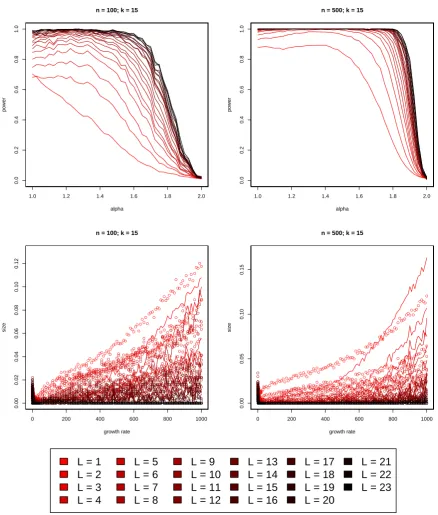
Figure 2: Comparison of the Poisson-fixed-
s
approximate likelihood ratio test with s = 50, and
the KDE approximation proposed in this article with
L
= 23 loci and lumping from
k
= 15.
The first row shows the empirical power of the test, and the second the empirical size with
ε
= 0
.
01. In the second row, red characters denote a true algebraic growth model, and black
characters denote a true exponential growth model. Results are presented under the assumption
of independent loci (“KDE” and“fixed
s
”) in which case each data set is treated as 1000
×
L
independent observations, and for a single SFS obtained by averaging all
L
loci (“Averaged
KDE” and “Averaged fixed
s
”). The sample sizes are
n
= 100 on the left and
n
= 500 on
the right. Post-processing the simulated data to obtain these graphs in
R
took 71 minutes
for
n
= 100, and 274 minutes for
n
= 500 on a single Intel i5-2520M 2.5 GHz processor. The
expected branch lengths for the Poisson-fixed-
s
methods were estimated from 100 000 coalescent
[image:10.595.75.515.202.633.2]
(11)

![Figure 2 shows that (5) substantially improves on the test of [Eldon et al., 2015] in terms of thepower to distinguish multiple merger coalescents from population growth](https://thumb-us.123doks.com/thumbv2/123dok_us/9430092.448397/10.595.75.515.202.633/figure-substantially-improves-thepower-distinguish-multiple-coalescents-population.webp)