How many parameters actually affect the mobility of conjugated polymers?

warwick.ac.uk/lib-publications

Original citation:

Fornari, Rocco P., Blom, Paul W. M. and Troisi, Alessandro. (2017) How many parameters actually affect the mobility of conjugated polymers? Physical Review Letters, 118. 086601.

Permanent WRAP URL:

http://wrap.warwick.ac.uk/98550

Copyright and reuse:

The Warwick Research Archive Portal (WRAP) makes this work by researchers of the University of Warwick available open access under the following conditions. Copyright © and all moral rights to the version of the paper presented here belong to the individual author(s) and/or other copyright owners. To the extent reasonable and practicable the material made available in WRAP has been checked for eligibility before being made available.

Copies of full items can be used for personal research or study, educational, or not-for-profit purposes without prior permission or charge. Provided that the authors, title and full bibliographic details are credited, a hyperlink and/or URL is given for the original metadata page and the content is not changed in any way.

Publisher statement:

© 2017 American Physical Society

A note on versions:

The version presented here may differ from the published version or, version of record, if you wish to cite this item you are advised to consult the publisher’s version. Please see the ‘permanent WRAP URL’ above for details on accessing the published version and note that access may require a subscription.

1

How many parameters actually affect the mobility of conjugated polymers?

Rocco P. Fornari,1 Paul W. M. Blom,2 Alessandro Troisi1

1_{Department of Chemistry, University of Warwick, Coventry CV4 7AL, United Kingdom}

2 _{Max Planck Institute for Polymer Research, Ackermannweg 10, 55128 Mainz, Germany}

Abstract

We describe charge transport along a polymer chain with a generic theoretical model depending in principle on tens of parameters, reflecting the chemistry of the material. The charge carrier states are obtained from a model Hamiltonian that incorporates different types of disorder and electronic structure (e.g. the difference between homo- and co-polymer). The hopping rate between these states is described with a general rate expression, which contains the rates most used in the literature as special cases. We demonstrate that the steady state charge mobility in the limit of low charge density and low fieldultimately depends on only two parameters: an effective structural disorder and an effective electron-phonon coupling, weighted by the size of the monomer. The results support the experimental observation [N. I. Craciun, J. Wildeman, and P. W. M. Blom,

Phys. Rev. Lett. 2008, 100, 056601] that the mobility in a broad range of (polymeric) semiconductors follows a universal behaviour, insensitive to the chemical detail.

The charge mobility in the now vast class of semiconducting polymers has proven itself very difficult to rationalize. Modest changes in the chemistry cause large variation in measured mobility and the space of possible parameters that can be explored (including molecular weight and processing) defied any attempt at truly predictive modelling. On the other hand, the essence of charge transport (temperature, field and charge carrier dependence) can be captured by fairly simple models depending on just few parameters [1-3]. The intriguing experiments of ref. [4] show that, for a large number of materials, the low-charge-density mobility  obeys a simple temperature dependence





0exp E k Ta B

   , where the parameter ₀ is universal for all materials and the only material-dependent parameter is the activation energy Ea (k TB is the thermal energy). It is certainly surprising that the chemical and morphological [5] complexity of organic semiconductors can be reduced to a single effective parameter for each material. In this work we consider a rather general model that should mimic the large parameter space encountered in realistic polymers and study how many distinct effective parameters actually affect the charge mobility, through a parameter space exploration. This approach is somewhat opposite with respect to the most common strategies that

start with a less general model that already contains a limited number of parameters (as in Gaussian disordered models [3] or mobility edge models [6] with four and two parameters, respectively). In particular, we allow (i) for a more general (and realistic) electronic structure and (ii) for a more general hopping rate expression.

2 electron phonon couplings interactions determine the hopping rates between these states [7,8]. We therefore first describe the disordered Hamiltonian in terms of a few parameters, then we introduce the models and parameters for the hopping rate and finally a model to describe the mobility.

In a realistic model for charge transport the delocalization of the single electron states must vary with energy because it was observed from atomistic simulations [9-11] (and expected from localization theories [12]) that states at the band edge are considerably more localized than states few k T_B from the edge. So, rather than assuming a density of states (DOS) and an independent constant localization length we generate the one-electron states involved in the transport by computing the eigenstates of a random electronic Hamiltonian [13]. This is defined for a polymer chain as

el 0

ˆ _

_

_{ }

_

_{  1 . .}

n n

n n

H n n n n h c (1)

n represents the transport-relevant orbital of the n-th monomer (site). The site energies

εn and the couplings τn between neighbouring sites are set to realistic values and they

include diagonal and off-diagonal disorder, respectively. An alternating copolymer structure can also be obtained by assigning different ranges of energies to even and odd sites. From the diagonalization of Hˆ₀el we obtain the wavefunctions _i0 _ni

nc n  



and the energies Ei of the electronic states. Starting from few realistic parameters

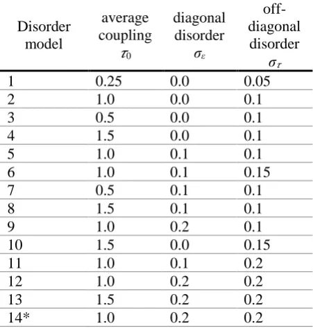
(energies, couplings and disorder), this model Hamiltonian naturally provides a detailed energy landscape of electronic states localized by static disorder (see Figure 1) and a realistic DOS. To illustrate the results of this work we consider 14 models of random Hamiltonian, different for the average (ε0 and𝜏0) and standard deviation (σε and σ𝜏) of the

[image:4.595.171.421.100.273.2]

3

Figure 1. Electronic energy landscape for the lowest energy eigenstates of a disordered polymer chain of 1000 monomers with periodic boundary conditions and parameters of model 5. Each eigenstate is represented by a horizontal segment centered on the site where c_ni2 is maximum, whose length is the localization length, defined as





1/2 2 2

2 n  n . The transitions between eigenstates which contribute most to the steady state mobility are represented by arrows. They are selected to make up 90% of the total particle velocity (definition given in the SI). One should note the increased delocalization at higher energy and the importance of delocalized states in promoting long range displacement of the carrier.

Table 1. Hamiltonian parameters in eV for different models of disorder labelled 1-14. ε0 is always 0.0 eV and defines the zero of our energy scale.

Disorder model

average coupling

𝜏0

diagonal disorder

σε

off-diagonal

disorder

σ𝜏

1 0.25 0.0 0.05

2 1.0 0.0 0.1

3 0.5 0.0 0.1

4 1.5 0.0 0.1

5 1.0 0.1 0.1

6 1.0 0.1 0.15

7 0.5 0.1 0.1

8 1.5 0.1 0.1

9 1.0 0.2 0.1

10 1.5 0.0 0.15

11 1.0 0.1 0.2

12 1.0 0.2 0.2

13 1.5 0.2 0.2

14* 1.0 0.2 0.2

[image:4.595.185.411.479.716.2]

4 The next step is to express the rate of hopping between the eigenstates of Hˆ₀el, a problem that was described in detail in ref. [8], with the main physical ideas summarized here. The transition between localized electronic states is caused by electron-phonon coupling terms. For an intuitive picture we can imagine that a displacement from the equilibrium position along one of these modes k with energy _kI linearly couples any two electronic states i and j with a coupling strength M_{ij k,} . The transition between states i and j can be therefore induced by mode k, which we call inducing mode. Following ref. [14] we incorporate the effect of the distance between initial and final states by parametrizing the coupling as _{ij k,} 2 _k2 _ni 2 _nj 2

n

M M



c c , i.e. states are coupled more if they overlap more. Without other electron-phonon coupling terms this transition is only possible between states whose energy difference is _kI because one phonon is always created or destroyed in the hopping process and the hopping rate would take the standard form [15]













2

I I I I

, ( ) 1  ( )



_

_

_

_

 



_       _

i j ij k k ij k k ij k

k

k M N E N E , (2)

with ΔEij being the electronic energy difference between the states, the summation

running over the inducing modes k; N is the boson occupation and  the Dirac delta. However, transitions between states with larger energy difference are possible via the exchange of multiple phonons with the system. These are the phonons associated with the relaxation of the nuclear geometry following the transition between states i and j, i.e. in the language of Marcus theory [16], those associated with the reorganization energy _ij for the hopping process. We have called these modes accepting as they can make up for larger energy difference between initial and final states; they are also the modes associated with polaronic effects. The resulting rate is a generalization of eq. (2) where the Dirac delta is replaced by a broader function, the Franck-Condon weighted density of states



_FCWT,ij

 

E :













2 I I FCWT, , I I FCWT,

( ) 1

( ) .

i j ij k k ij ij k

k

ij ij

k k

k M N E

N E



_

_

_

 



 _         



(3)

The analytical expression for



_FCWT,ij

 

E is more manageable if one makes the customary assumption that _ij _ij(C)+_ij(Q), i.e. that the reorganization energy is the sum of a classical component due to low frequency modes _ij(C)=(1 f_Q)_ij, and a quantum component _ij(Q)=f_Q_ij, due to one effective mode with energy A [17]:

 

2

FCWT, (C) , '

' B

1

( ) FC

4





 





ij ij ww

w w

ij

E P w

5 (C) A ( 2 C) B ( ( ' ) ) exp 4                 ij ij

E w w

k T . (4)

In eq. (4), w and w’ are the vibrational quantum numbers of the accepting mode in the initial and final states, P(w) the Boltzmann population in the initial state and FC_{ij ww, '} the Franck-Condon integrals (explicitly given in the SI and depending on



_ij(Q)). It was shown [8], that the rate expression Error! Reference source not found. is extremely general as it can be reduced to Miller-Abrahams [18], Marcus [16], Marcus-Levich-Jortner [17] or Vukmirovic [15] rates when the appropriate limits are taken.

The total reorganization energy _ij depends on the delocalization of both states i and j

through the relation _ij ₁



IPR_i IPR_j



1, where





1 4 ( ) ( ) IPR  



i j _n cni j is the inverse participation ratio of state i(j) (a measure of how many sites share the charge) and ₁ is the reorganization energy for the removal of a carrier from a single site. Note that, in the limit ₁0 of hopping between delocalised states, eq. 3 becomes identical to eq. 2 as expected. The role of the accepting modes is therefore determined by the material dependent parameters₁, A and f_Q.

Given a set of hopping rates the mobility can be computed in several ways. Here we use an adaptation of the method originally proposed in [19] with the detail given in [7] and the SI, based on evaluating the steady state solution of the master equation in the limit of low field and low carrier density (i.e. ignoring inter-carrier Coulombic interactions [20]). We will compare with experimental data extrapolated to the same limit, while generalizations, including to non-equilibrium situations, would be possible within the model but are not considered here. We ignore the role of inter-chain hopping, which has been shown to be correct for polymers with very long persistence length [21], with means to extend the results to the general case recently proposed in [13] at the cost of additional parameters in the model. These corrections could become more significant if the inter-chain hopping had substantially different transport characteristics from the intra-chain one. However, experiments on aligned thin films indicate no anisotropy of mobility [22] (and activation energy [23]), supporting the approximation proposed here in the first instance. To evaluate the mobility one needs to introduce the distance between monomers d as an additional model parameter, which we initially set to a value of the correct order of magnitude, 1 nm, while the role of this parameters is further discussed below.

To summarize, the model incorporates (i) parameters of the electronic Hamiltonian that determine DOS and localization characteristics (𝜏0, σε,σ𝜏), (ii) parameters determining

the local electron phonon coupling (₁, A, fQ), (iii) parameters determining the

non-local electron phonon coupling (the set of _kI andM_k), (iv) the inter-monomer distance

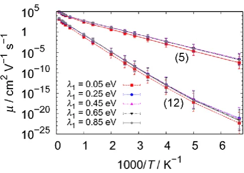
6 The role of ₁ on the mobility is virtually negligible on the ( )T curves, as shown in Figure 2 for the electronic Hamiltonian models 5 and 12. The result is due to the fact that polaronic effects are negligible when the transport is mediated by fairly delocalized states (which have a negligible reorganization energy), an assumption implicit in many of the models proposed so far, which is therefore validated by our more general model. This observation is in contrast with the extremely important role attributed to ₁ in works considering the hopping rate between small molecules [24]. The limited importance of polaronic effects makes completely unimportant also the parameters that control their detail, i.e. A and fQ (see also Figures S3 and S4 in the SI). For the remainder of this

work, we have set the relevant parameters to realistic values: ₁ = 0.45 eV [25], A

= 0.198 eV, fQ = 0.4 [8]).

Figure 2. Mobility as a function of temperature computed using different values for the reorganization energy of the single site ₁. Results are shown for disorder models 5 and 12 (but are similar for any disorder model). They are computed with model (a) (see caption of Figure 3) for the inducing modes electron-phonon coupling.

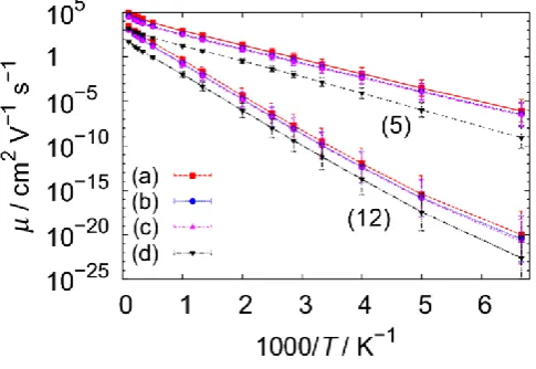
The inducing modes participate to the rate expression (2) or (3) through the mode frequencies _kI and coupling strengths M_k2 and there are in principle many conceivable possibilities. However, we show in Figure 3 that the ( )T curves do not change much if we consider different combinations of low and high frequency inducing modes, provided that



M_k2 is kept constant. In particular, the differences between the different distributions of kI values are negligible if one excludes the very unphysical model where there is a single high frequency inducing mode. The numerical results suggest that one can capture the variability between chemical systems simply by considering only one low frequency inducing mode (model (a) in Figure 3), and therefore a single parameter M2 (now dropping the suffix k) that is essentially a measure of how effectively the nuclear motions mix the electronic states. The parameter M2 _{is ultimately just a}

[image:7.595.167.410.287.459.2]

7 distance between sites d2_{, the product d}2_M2 _{can be taken as one single effective}

[image:8.595.168.411.163.330.2]

parameter directly proportional to the mobility and the only relevant parameter beside those defining the electronic Hamiltonian in Eq. (1). To obtain realistic ranges of mobilities with the choice of d equal to 1 nm, the results are presented with M set to 2.0 · 10-4 eV. However, the conclusions do not depend on this pair of choices.

Figure 3. Mobility as a function of temperature for disorder models 5 and 12 computed using four different models for the inducing modes. The inducing mode frequencies _kI and coupling strengths M_k2 have been set as follows. Model (a): one low energy mode (6.2 meV); model (b): four modes from low to intermediate energy (6.2, 12.4, 37.2, 49.6 meV); model (c): five modes from low to high energy (6.2, 12.4, 37.2, 49.6, 186 meV); model (d): one high energy mode (186 meV). The values ofM_k2 have been chosen to be identical for all inducing modes with strength such that



_kM_k2= 4.0 · 10-8 _eV2 _{to reproduce the experimental range of mobilities.}

8

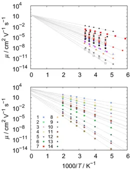
Figure 4. Top: experimental hole mobility vs. 1/T for a range of organic semiconductors, adapted from ref. [4] and augmented with additional data points [26]. Bottom: mobility vs. 1/T

from various models of chains of 1000 monomers with a variety of disorder parameters (see Table 1), including an alternating copolymer (model 14). The lines are obtained from a least squares linear fitting of log µ vs. 1000/T.

The results of the model are strikingly similar to the experimental results reported by Blom et al. [4,26] for a broad range of chemically different organic semiconductors and also reported in Figure 4. All experimental data can be fitted by an Arrhenius temperature dependence   ₀exp



E k Ta _B



at low field and low charge density. There seems to be a common infinite temperature mobility μ0 = 30 cm2V-1s-1 valid for

[image:9.595.147.409.75.418.2]

9 According to our model, 

 

T only depends on two parameters, a combined effect of disorder (which determines the activation energy) and the weighted strength of the electron-phonon coupling, d2M2, acting as a pre-factor for our computed mobility. To fully account for the experimental observation we can speculate that the parameter d2M2

is approximately a constant for this class of materials. The scaling of d and M supports this idea. One can partition the polymer into nearest neighbour interacting sites in different ways, e.g. considering a smaller or larger unit to take as “the monomer”, and this partition defines the other parameters of the model. According to the definition of

M, the product dM should remain constant in order to have consistent models with different definitions of the monomer length, e.g. if we consider larger monomers, the effect of inducing modes will be weaker. As we have noted when we discussed the negligible importance of reorganization energy, the most effective charge hopping events involve fairly delocalized states (tens of monomers) and it is therefore not surprising that the electron-phonon coupling terms, being averaged over a large portion of the material, become weakly dependent on the chemical detail for similar classes of compounds. Intuitively, the hopping is promoted by low frequency modes that alter the energy and coupling between the π-conjugated segments. The most relevant modes are out-of-plane and torsional modes of the carbon backbone.

In conclusion, we performed a parameter space exploration of a generic charge transport model suitable for realistic polymers in the limit of low charge density and electric field. We have found that the temperature dependence of the mobility of conjugated polymers is determined by just two effective parameters, even though the model itself depends in principle on many tens of parameters. Remarkably, we find that polaronic effects, very different from system to system, are irrelevant for the computed mobility. The model helps explaining the experimental observation of a universal temperature dependence of the mobility determined by a single experimental parameter. To fully account for the experimental observation we have tentatively speculated that the strength of the mixing between electronic states due to the inducing modes is similar across all materials considered.

10

References

[1] H. Sirringhaus, Adv. Mater. 17, 2411 (2005).

[2] N. Tessler, Y. Preezant, N. Noam Rappaport, and Y. Roichman, Adv. Mater. 21, 2741 (2009).

[3] H. Bässler, Phys. Status Sol. B 175, 15 (1993).

[4] N. I. Craciun, J. Wildeman, and P. W. M. Blom, Phys. Rev. Lett. 100, 056601 (2008).

[5] D. Mendels and N. Tessler, Scientific Reports 6, 29092 (2016).

[6] R. A. Street, J. E. Northrup, and A. Salleo, Phys. Rev. B 71, 165202 (2005). [7] R. P. Fornari and A. Troisi, Phys. Chem. Chem. Phys. 16, 9997 (2014). [8] R. P. Fornari, J. Arago, and A. Troisi, J. Chem. Phys. 142, 184105 (2015). [9] J. M. Frost, J. Kirkpatrick, T. Kirchartz, and J. Nelson, Farad. Discuss. 174, 255 (2014).

[10] T. Qin and A. Troisi, J. Am. Chem. Soc. 135, 11247 (2013). [11] T. Liu and A. Troisi, Adv. Funct. Mater. 24, 925 (2014). [12] N. F. Mott, Proc. R. Soc. Lond. A 345, 169 (1977).

[13] R. Noriega, A. Salleo, and A. J. Spakowitz, Proc. Natl. Acad. Sci. USA 110, 16315 (2013).

[14] N. Vukmirovic and L.-W. Wang, Appl. Phys. Lett. 97, 043305 (2010). [15] N. Vukmirovic and L.-W. Wang, Nano Letters 9, 3996 (2011).

[16] R. Marcus, J. Chem. Phys. 24, 966 (1956). [17] J. Jortner, J. Chem. Phys. 64, 4860 (1976).

[18] A. Miller and B. Abrahams, Phys. Rev. B 120, 745 (1960).

[19] Z. G. Yu, D. L. Smith, A. Saxena, R. L. Martin, and A. R. Bishop, Phys. Rev. B

63, 085202 (2001).

[20] J. J. M. van der Holst, F. W. A. van Oost, R. Coehoorn, and P. A. Bobbert, Phys. Rev. B 83, 085206 (2011).

[21] P. Carbone and A. Troisi, J. Phys. Chem. Lett. 5, 2637 (2014).

[22] C. Tanase, P. W. M. Blom, and D. M. de Leeuw, Phys. Rev. B 70, 193202 (2004). [23] C. Tanase, E. J. Meijer, P. W. M. Blom, and D. M. de Leeuw, Phys. Rev. Lett.

91, 216601 (2003).

[24] J. L. Bredas, D. Beljonne, V. Coropceanu, and J. Cornil, Chem. Rev. 104, 4971 (2004).

[25] R. P. Fornari and A. Troisi, Adv. Mater. 26, 7627 (2014).

[26] M. Kuik, G.-J. A. H. Wetzelaer, H. T. Nicolai, N. I. Craciun, D. M. De Leeuw, and P. W. M. Blom, Adv. Mater. 26, 512 (2014).