Conceptual data sampling for breast cancer histology image classification

warwick.ac.uk/lib-publications

Original citation:

Rezk, Eman, Awan, Zainab, Islam, Fahad, Jaoua, Ali, Al Maadeed, Somaya, Zhang, Nan, Das, Gautam and Rajpoot, Nasir M.. (2017) Conceptual data sampling for breast cancer histology image classification. Computers in Biology and Medicine, 89. pp. 59-67.

Permanent WRAP URL:

http://wrap.warwick.ac.uk/90844

Copyright and reuse:

The Warwick Research Archive Portal (WRAP) makes this work by researchers of the University of Warwick available open access under the following conditions. Copyright © and all moral rights to the version of the paper presented here belong to the individual author(s) and/or other copyright owners. To the extent reasonable and practicable the material made available in WRAP has been checked for eligibility before being made available.

Copies of full items can be used for personal research or study, educational, or not-for-profit purposes without prior permission or charge. Provided that the authors, title and full bibliographic details are credited, a hyperlink and/or URL is given for the original metadata page and the content is not changed in any way.

Publisher’s statement:

© 2017, Elsevier. Licensed under the Creative Commons

Attribution-NonCommercial-NoDerivatives 4.0 International http://creativecommons.org/licenses/by-nc-nd/4.0/

A note on versions:

The version presented here may differ from the published version or, version of record, if you wish to cite this item you are advised to consult the publisher’s version. Please see the ‘permanent WRAP URL’ above for details on accessing the published version and note that access may require a subscription.

1

Conceptual Data Sampling For Breast Cancer Histology Image

Classification

Eman Rezka

,

,

,

Nan Zhangb, Gautam Dasc, Nasir Rajpootd

a_{Department of Computer Science and Engineering, Qatar University, Qatar}

b _{Department of Computer Science, George Washington University, USA}

c _{Department of Computer Science and Engineering, University of Texas at Arlington, USA}

d _{Department of Computer Science, University of Warwick, UK}

2 Abstract

Data analytics have become increasingly complicated as the amount of data has increased. One technique that is used to enable data analytics in large datasets is data sampling, in which a portion of the data is selected to preserve the data characteristics for use in data analytics. In this paper, we introduce a novel data sampling technique that is rooted in formal concept analysis theory. This technique is used to create samples reliant on the data distribution across a set of binary patterns. The proposed sampling technique is applied in classifying the regions of breast cancer histology images as malignant or benign. The performance of our method is compared to other classical sampling methods. The results indicate that our method is efficient and generates an illustrative sample of small size. It is also competing with other sampling methods in terms of sample size and sample quality represented in classification accuracy and F1 measure.

Keywords: Data sampling; Formal concept analysis; Image segmentation; Breast cancer

classification; histopathology.

1. Introduction

3

as malignant or benign. It is here that the importance of sampling arises to take a discriminative set of the data to be used in the classification process.

The objective of any data sampling technique is to extract a portion of the data that preserves data behavior while reducing sampling cost and error [2]. In this paper, a new data sampling method is proposed and employed in classifying breast cancer images. This method is rooted in formal concept analysis (FCA) theory, which is a mathematical framework used for conceptual data analysis, in which data are represented as a binary relation that links tuples and features [3]. This binary relation is transformed into a set of binary patterns, which is then used to select a sample from the data while preserving patterns proportions across the data.

The novelty of the sampling method is due to several factors: 1) it considers all data features while generating patterns, unlike other existing sampling methods that consider only one feature; 2) it considers data distribution among different patterns to generate proportional samples that represent the real distribution of data; 3) it does not require any prior knowledge about the data.

4

The paper is organized as follows; section 2 introduces some background information. Section 3 explains the methodology including image processing, sampling and learning steps. In section 4, the data set, experimental setup, and experimental results are discussed. Finally, we conclude our work.

2. Background

In this section, the backgrounds of the topics examined in the subsequent sections are described in detail.

2.1 Formal Concept Analysis

FCA is a mathematical framework built on lattice theory that provides data analysis and knowledge discovery [3]. It works by analyzing the binary relations between tuples and features [4]. FCA is a beneficial data analysis technique that has been widely applied in different fields such as feature reduction [5], image mining [6], and decision-making [7]. In FCA, the main entity is a binary relation that is called a formal context, which is defined as follows: A formal context (FC) is a triplet k = <O,A,I>, where O and A represent objects and attributes respectively. The binary relation defined between O and A is noted as I and the term I(o, a) means the value of object o in attribute a [8], [9], [10].

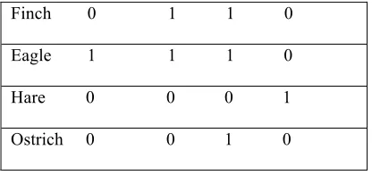
Table 1 provides an example of a formal context with O = {Lion, Finch, Eagle, Hare, Ostrich}, A = {Preying, Flying, Bird, Mammal} and I (Finch, Bird) = 1.

Table 1. Example of a formal context

Preying Flying Bird Mammal

5

Finch 0 1 1 0

Eagle 1 1 1 0

Hare 0 0 0 1

Ostrich 0 0 1 0

2.2 Sampling Methods

One way to overcome the data size problem is data sampling, which is the process of drawing a sample from a population that helps in making inferences. The process of drawing a sample is shown in Fig. 1. The accuracy of the analytics performed using only samples of the data is extensively based on the quality of the selected samples. Therefore, the sampling design plays a crucial role in both the sampling process and the inference process. As the sampling design provides the method used to collect the sample, it should be accurate, efficient, and feasible [11]. In this paper, we use simple random sampling and stratified sampling for their simplicity and efficiency.

6 2.2.1 Simple Random Sampling (SRS)

All elements in the population have equal probability of being selected for the sample. SRS is easy to implement and it can be used to estimate the population total and mean. The mean is unbiased and sample variance can be estimated using a single sample. However, it is not efficient enough [12], [13].

2.2.2 Stratified Sampling

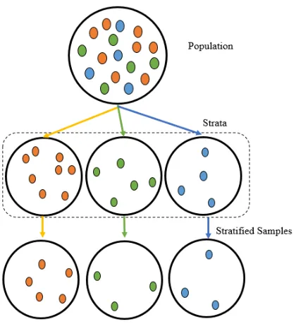
In stratified sampling, the population is divided into non-overlapping groups based on certain known criteria such as age, gender, or country. This set of groups is called strata, and each subgroup is called a stratum. A sample is drawn randomly from each stratum [14]. The process of stratified sampling is shown in Fig. 2.

7

Fig. 2. Stratified sampling

2.3 Image Segmentation

8

Fig. 3. Breast cancer image segmentation [16]

Numerous methods are developed to segment the images. In [16], breast cancer images segmentation is represented as a machine learning problem that is solved using supervised and unsupervised learning methods. Gurcan et al. in [18] target segmenting the hematoxylin and eosin (H&E) stained images to classify a pediatric nervous system cancer. They integrated the top hat and thresholding algorithms to segment the cell nuclei. Cosatto et al. provide a high accuracy classifier for breast cancer nuclear segmentation and grading [19]. Yang et al. segment the blood cancer histopathology specimens by constructing a concave vertex graph. This graph is based on employing a contouring model to define the concave boundary points and inner edges [20]. For breast cancer images of tissue microarrays, Qi et al. succeeded in accurately segmenting overlapped cells. Their model started by finding the object centers, then clustering, and finally contouring the cells [21].

9

classical active contouring algorithm to segment the highly overlapped objects of breast and prostate tissues. Their proposed technique is able to generate better boundary separations and handle object occlusion. In [24], a framework for classifying breast cancer image pixels as tumor or stromal regions is proposed. The image is split into four regions: tumor, Hypocellular stroma, Hypercellular stroma, and fat that is removed during the preprocessing step. The texture features of the hypo and hyper stroma are extracted using different orientations of a Gabor filter.

The emergence of deep learning helped the improvement of image segmentation and analysis. Sirinukunwattana et al. [25] propose an integrated framework for nuclei detection and classification that is based on deep learning techniques. A convolutional neural network is mainly employed for both detection and classification. In [26], the authors employ a convolutional neural network to solve the problem of classifying unbalanced data of breast cancer images. The proposed framework segments the images, and then recognizes the non-mitotic parts of the image that are later under sampled, while oversampling the mitotic parts to achieve the balance between the classes.

3. Methodology

10

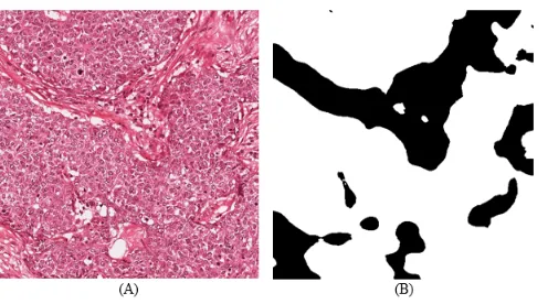
In Fig. 4, image (A) shows the original breast cancer image, while image (B) is the predicted one resulting after the learning process; the white regions represent the tumors and the black regions are the normal cells.

Fig. 4. Example of the original breast cancer image (A) and the predicted one (B)

3.1 Image Processing

In image processing, the image quality is improved through: 1) stain normalization, 2) conversion to gray scale, and 3) noise removal.

11

The stained images are converted to grey scale using MATLAB2_{. Then, the noise in the} images is removed by smoothing the image brightness using a smoothing Gaussian filter that fits the image distribution, Fig. 6 illustrates a source colored breast cancer image (A) and a preprocessed image after stain normalization, grey scale conversion, and noise removal (B).

Fig. 5. Illustration of stain normalization on breast cancerimages [16]

(A) (B)

12

Fig. 6. The difference between the source and preprocessed image [16]

After preprocessing images, a feature extraction step is performed. Features represent the characteristics of the images. In this work only the textural features are extracted to minimize color and intensity dependencies. Textural features depend on the structure and the pattern of the tumor regions and hence, they are dominant in determining the tumor and non-tumor regions of an image.

Several techniques can be used to extract textural features such as Maximum Response 8 (MR8) filter bank [30], Root Filter Set (RFS) bank [31], and Haralick filter [32]. In this work, we focus on the MR8Fast filter that is derived from the MR8 filter bank. It extracts 8 responses only, so each image has 8 features.

3.2 The Proportional Sampling

13

Fig. 7. Proposed sampling method

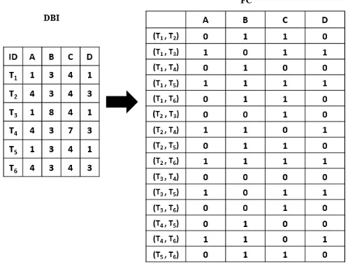
A. Convert Data to Formal Context

Data are converted to the formal context by performing pairwise comparisons between data tuples as in [33]. Fig. 8 shows the example of a database instance (DBI) that is transformed into a formal context. Tuples T1 and T2 are compared for attributes A, B, C, and D. This

comparison is translated into a new object in the FC with the same attributes containing “0” if the values are not equal and “1” otherwise. Tuple T1(A) is not equal to T2(A); hence,

(T1,T2) (A) in the FC is “0”. However, T1(B) = T2(B), so (T1,T2) (B) in the FC is “1”.

Fig. 8. Converting database instance into a formal context

14 𝑆𝑖𝑚𝑖𝑙𝑎𝑟𝑖𝑡𝑦 = 1−_!"#!!!!_!!,!_!! (1)

where n1, n2 are the two numbers.

In this step, the percentage of similarity is calculated during the pairwise comparison. If the similarity between the data values is greater than a certain threshold, then the FC object value is “1”; otherwise the value of the FC object is “0”.

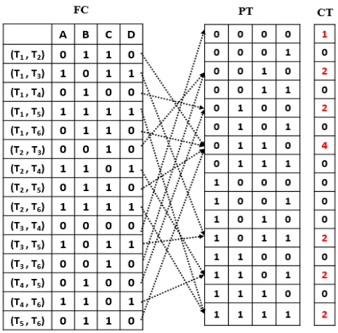
B. Map to Binary Patterns

A set of binary patterns is generated based on the number of features in the FC which is the same as the number of features of the dataset. A formal context with M features has a binary pattern table of size 2M patterns. Each FC object is mapped to one of these patterns and a counter attached to each pattern is incremented. Only a fixed number of FC objects is stored for each pattern to minimize memory usage. Examples of a binary pattern table (PT) and the counter table (CT) generated for a FC with four attributes are illustrated in Fig. 9. For example, since objects (T2, T3) and (T3, T6) are mapped to pattern “0010”, its

15

Fig. 9. Mapping FC objects to patterns

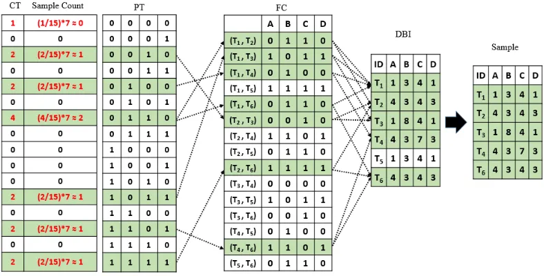
C. Calculate Pattern Proportions

After mapping all FC objects to their corresponding patterns, the CT indicates the frequencies of each pattern across all the data. Each value in the CT is divided by the total number of objects in the formal context to obtain the proportion of each pattern. This proportion is multiplied by a multiplier K where K > 0.It controls the number of objects to be sampled from each pattern. The higher the multiplier value, the bigger the sample size. It is calculated as follows:

𝑃𝑎𝑡𝑡𝑒𝑟𝑛𝑃𝑟𝑜𝑝𝑜𝑟𝑡𝑖𝑜𝑛 =_!"#$%&!" (!"##$%&_{!" !" !"#$%&'})

16

A number of objects is selected from each pattern based on its calculated sample size. For example, a pattern sample count of 10 means that the first 10 objects belonging to this pattern are selected as the sample.

D. Map Objects to Original Data

The pattern sample size provides statistical information about the tuples in the original database. Patterns with higher proportions have higher numbers of FC objects and thus, more objects are sampled from them while patterns with low proportions and zero sample size are not included in the sample. This mapping process significantly empowers our sampling method because it recognizes the outliers and data distribution in different patterns without prior knowledge about the data.

The sampled FC objects are mapped to the tuples in the original database to generate the sample. For example, in Fig. 10, the pattern {0110} has four objects {(T1, T2), (T1, T6), (T2,

T5) and (T5, T6)}. In this example, the multiplier is 7 to get a very small sample because the

dataset is already fairly small. The pattern sample size for {0110} is 1.87, which can be rounded to 2 for the sample count, so two FC objects are randomly selected from this pattern. Assume that FC objects {(T1, T2) and (T1, T6)} are sampled from the FC.

Therefore, the tuples T1, T2, and T6 are selected from the original dataset in the sample.

17

Fig. 10. Sampling from DBI based on pattern proportion

3.3 The Learning Process

The generated samples are used to classify the image pixels as malignant or benign. This is achieved by a machine learning process based on 5 classification algorithms: naïve Bayes (NB), support vector machine (SVM), pattern net (PN), cascade forward net (CFN), and feed forward net (FFN) using the statistics and machine learning toolbox of MATLAB3_.

18

The training set is the sample and the test set is not previously known to the classifier. The classification accuracy and F1 measure [34] are reported to evaluate the samples and the learning process. In addition, our sampling method is compared to the classical sampling methods; simple random sampling (SRS) and stratified sampling (SS). All the generated samples are used through the learning process for validation and evaluation.

4. Results and Discussion

In this section, we discuss the experiments performed on the breast cancer images of the MITOS 2012 dataset4_{. It contains 50 images from 5 patients and each image has 512 × 512}

pixels and 8 features that are labelled (malignant or benign) manually by domain experts. The experimental setup section explains the configurations of each group of experiments; the data split and cross validation results sections show the results achieved using the clarified configurations.

4.1 Experimental Setup

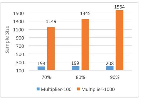
Two main groups of experiments are performed, the data split group and the cross-validation group. In the data split experiments, the 50 images are divided into 2 equal sized partitions. A random sample of size 10,000 pixels is selected from the first partition that includes 25 images (400 pixels from each image) and given as input for all sampling methods. The second partition with the other 25 images is used for testing with a total size of 6,553,600 (512 x 512 x 25) pixels. The proposed sampling method, PPS is configured with 70%, 80%, and 90% similarity thresholds to study their effects on the sample quality. Also the multiplier is tuned to 100 and 1000 to produce different sample sizes. On the other

19

hand, SRS and SS methods are tested for sample sizes of 200 and 1500. The results of the data split experiments are discussed in section 4.2.

In the cross-validation group, the images are subdivided into 10 sets of 5 images. From each image, a smaller sample of 750 rows is randomly selected, thus, each subset has a total sample size of 3750(750*5) rows. Since we are doing 10-fold cross-validation, 9 subsets are used for training while one is used for testing and the input to PPS is the 9 subsets combined into a single dataset totaling 33,750 rows. The PPS similarity threshold is tuned to 70%, 80%, and 90% just like in the previous experiment while the multiplier is set to 1000 to have sufficient sample size. On the other hand, SRS and SS are configured with a sample size of 1200 rows. The results of the cross-validation experiments are discussed in section 4.3.

4.2 Data Split Results

20

Fig. 11. Sample size with all similarity thresholds and multipliers

The comparison of the algorithms using different similarity thresholds and multiplier-100 are shown in Fig. 12 and Fig. 13. SVM outperforms other algorithms especially for the 70% similarity threshold sample that leads in terms of accuracy and F1 measure.

Fig. 12. Accuracy of all algorithms and similarity thresholds

Fig. 13. F1 of all algorithms and similarity thresholds

193 199 208

1149 1345 1564 100 300 500 700 900 1100 1300 1500

70% 80% 90%

Sam

pl

e

Si

ze

Mul=plier-100 Mul=plier-1000

66 68 70 72 74 76 78 80

NB SVM PN CFN FFN

Ac cu rac y % Mul=plier-100

70% 80% 90%

.72 .74 .76 .78 .80 .82 .84 .86

NB SVM PN CFN FFN

F1 Me as ur e Mul=plier-100

21

In addition, we also compared the accuracy and F1 measure using multiplier-1000 that are represented in Fig. 14 and Fig. 15. Here also, SVM outperforms all other algorithms but the differences in accuracy and F1 measure are not significant across the three similarity thresholds.

Fig. 14. Accuracy of different algorithms and similarity thresholds

Fig. 15. F1 Measure of different algorithms and similarity thresholds

Fig. 16 and Fig. 17 compare PPS with other sampling methods in terms of classification accuracy using the smaller and bigger sample sizes respectively. Fig. 18 and Fig. 19 represent the F1 measure using the smaller and bigger sample sizes. It is clear that PPS-100 is outperforming 200 and SS-200. Also, the accuracy of PPS-1000 is better than SRS-1500 and SS-SRS-1500. In addition, we also noticed the trend that the accuracy of all sampling methods improves with the increase in sample size. PPS-1000 gives the best accuracy and F1 measure when compared to SRS and SS using samples of size 200 and 1500. For example, PPS-100 using SVM achieved 78.9% accuracy with sample size 193 compared to 77% for SRS-1500 and 77.1% for SS-1500. Moreover, the F1 measure graph also shows that PPS is better than other methods. For example, using SVM, PPS-100 achieves 0.85 F1 measure with 193 sample size, while SRS-1500 and SS-1500 have an F1 measure of 0.83.

66 68 70 72 74 76 78 80

NB SVM PN CFN FFN

Ac cu rac y % Mul=plier-1000

70% 80% 90%

.70 .75 .80 .85 .90

NB SVM PN CFN FFN

F1 Me as ur e Mul=plier-1000

22

Fig. 16. Accuracy of all sampling methods using the smaller sample size

Fig. 17. Accuracy of all sampling methods using the bigger sample size

Fig. 18. F1 measure of all sampling methods using the smaller sample size

Fig. 19. F1 measure of all sampling methods using the biggersample size

4.3 Cross Validation Results

The comparison of the classification accuracy using different similarities and algorithms are shown in Fig. 20. The 90% similarity threshold results in the best classification accuracy for all algorithms while SVM outperforms all other algorithms with 78% accuracy. The F1 measure graph is shown in Fig. 21. It also confirms that the 90% similarity threshold is the best for this set of experiments. Also, SVM is achieving the best F1 measure with 0.84.

60 65 70 75 80

NB SVM PN CFN FFN

Ac

cu

rac

y

%

SRS-200 SS-200 PPS-100

65 70 75 80

NB SVM PN CFN FFN

Ac

cu

rac

y

%

SRS-1500 SS-1500 PPS-1000

.60 .65 .70 .75 .80 .85

NB SVM PN CFN FFN

F1

Me

as

ur

e

SRS-200 SS-200 PPS-100

.60 .65 .70 .75 .80 .85

NB SVM PN CFN FFN

F1

Me

as

ur

e

23

Fig. 20. Accuracy of the cross validation process Fig. 21. F1 measure of the cross validation process

In Fig. 22, we compare PPS with SRS and SS. We see that our proposed method is competing with the other sampling methods. SVM results in the highest accuracy compared to other classification algorithms with a value of 78%. In the F1 measure graph shown in Fig. 23, using NB algorithm, the PPS method is outperforming other methods. While using SVM, there is a slight difference in F1 measure between all the methods; SRS has value of 0.845, SS has 0.843, and PPS has 0.839.

Fig. 22. Accuracy of PPS against SRS and SS with the cross validation process

Fig. 23. F1 measure of PPS against SRS and SS with the cross validation process

68 70 72 74 76 78 80

NB SVM PN CFN FFN

Ac

cu

rac

y

%

70% 80% 90%

.60 .65 .70 .75 .80 .85

NB SVM PN CFN FFN

F1

Me

as

ur

e

70% 80% 90%

68 70 72 74 76 78 80

NB SVM PN CFN FFN

Ac

cu

rac

y

%

SRS SS PPS

.60 .65 .70 .75 .80 .85

NB SVM PN CFN FFN

F1

Me

as

ur

e

24 4.4Comparison with Other Methods

The proposed sampling method is compared to the SRS and SS. The results show that the PPS method is competing with the other techniques using different machine learning algorithms. In some cases, PPS is not outperforming SRS or SS especially when using CFN and FFN. For example, in Fig. 23 the F1 measure for PPS using FFN is 0.83 while SRS and SS have F1 measure of 0.84. This situation happens because of the lack of randomization when selecting the samples from the patterns. On the other hand, both SRS and SS employ randomization that can significantly improve the accuracy of methods that suffer from local minima and poor generalization, such as neural networks [35]. Moreover, SS can only be applied after analyzing the whole dataset and deciding the stratification parameters and stratum sizes whereas, both PPS and SRS don’t need any prior knowledge about the dataset.

25

In our work, we used the MITOS 2012 dataset that has been widely used in literature. Most of the work applied on this dataset focus on enhancing the accuracy of the classifiers by improving the input features or using advanced machine learning algorithms. In our framework, the main focus is enhancing the quality of the training data. This is achieved by applying the PPS sampler that considers data distribution among the patterns, therefore it can handle data skewness. The samples used in the learning process results in an average F1 measure of 0.84 for both data split and cross validation experiments.

In comparison Noorul et al. [26] proposed a two-phase model that handles class biasness using a balanced convolutional neural network. It is applied on the MITOS 2012 dataset and achieved an average F1 measure of 0.72. Irshad et al. [37] achieved F1 measure of 0.72 while detecting mitosis in breast cancer images. They focused on enhancing data features using selective color channels and employed SVM and decision tree algorithms for the learning. Ciresan et al. [38] achieved F1 measure of 0.66 using the same dataset while applying random undersampling technique with a deep neural network algorithm. Wang et al. [39] improved the features by combining handcrafted and convolutional neural network features. The F1 measure achieved is 0.73. Malon et al. [40] achieved F1 measure of 0.53 while integrating color, texture, and shape features with convolutional neural network extracted features.

5 Conclusion

26

a machine-learning case study of breast cancer images. Our method proved to be competitive with the other methods using different learning configurations. Moreover, it perfectly fits the unbalanced data used for classification because it generated a well-balanced sample of these data using the binary distribution. Additionally, it doesn’t require any prior knowledge about data or class distribution and it generates the patterns based on all attributes. Furthermore, PPS can be easily improved by employing randomization while selecting the objects from the patterns. This will allow our technique to fit more with machine learning algorithms that suffer from poor generalization such as neural networks. Feature selection algorithms can also be used to reduce the number of features incorporated in the pattern table to reduce the space complexity.

Acknowledgement

This contribution was made possible by NPRP grant #07- 794-1-145 from the Qatar National Research Fund (a member of Qatar Foundation). The statements made herein are solely the responsibility of the authors.

References

[1] Susan G. Komen, Breast Cancer Global Statistics | Susan G. Komen®, (n.d.).

http://ww5.komen.org/BreastCancer/Statistics.html (accessed February 8, 2017).

[2] Y. Su, G. Agrawal, J. Woodring, K. Myers, J. Wendelberger, J. Ahrens, Effective and

efficient data sampling using bitmap indices, Cluster Comput. 17 (2014) 1081–1100.

doi:10.1007/s10586-014-0360-5.

[3] R.W. Bernhard Ganter, Formal Concept Analysis, Mathematical Foundations, Springer,

27

[4] J. Baixeries, M. Kaytoue, A. Napoli, Characterizing functional dependencies in formal

concept analysis with pattern structures, Ann. Math. Artif. Intell. (2014) 1–21.

doi:10.1007/s10472-014-9400-3.

[5] W. Li, L. Wei, Data Dimension Reduction Based on Concept Lattices in Image Mining,

2009 Sixth Int. Conf. Fuzzy Syst. Knowl. Discov. (2009) 369–373.

doi:10.1109/FSKD.2009.685.

[6] Q.X.Q. Xiao, K.Q.K. Qin, Z.G.Z. Guan, T.W.T. Wu, Image mining for robot vision based

on concept analysis, 2007 IEEE Int. Conf. Robot. Biomimetics. (2007) 207–212.

doi:10.1109/ROBIO.2007.4522161.

[7] L. Yang, Y. Xu, Decision Making with Uncertainty Information Based on Lattice-Valued

Fuzzy Concept Lattice, J. Univers. Comput. Sci. 16 (2010) 159–177.

[8] Q. Wan, L. Wei, Approximate concepts acquisition based on formal contexts,

Knowledge-Based Syst. 75 (2015) 78–86. doi:10.1016/j.knosys.2014.11.020.

[9] I. Nafkha, A. Jaoua, Using Formal Concept Analysis for Heterogeneous Information

Retrieval, Cla 2005. (2005) 107–122. http://ceur-ws.org/Vol-162/paper10.pdf.

[10] S.O. Kuznetsov, Learning of Simple Conceptual Graphs from Positive and Negative

Examples, Princ. Data Min. Knowl. Discov. SE - 47. 1704 (1999) 384–391.

doi:10.1007/978-3-540-48247-5_47.

[11] B.M. Steele, Sampling Design and Statistical Inference for Ecological Assessment, A

Guideb. Integr. Ecol. Assessments. (2001) 79–91.

[12] Y. Tille, Sampling Algorithms, Springer, New York, 2006. doi:10.1007/978-0-387-98135-2.

28

Netherlands, 2011. doi:10.1007/978-90-481-9757-6.

[14] R. Benedetti, F. Piersimoni, P. Postiglione, Sampling Spatial Units for Agricultural Surveys,

Springer, Berlin, 2015. doi:10.1007/978-3-662-46008-5.

[15] A.C. Kulshreshtha, Basic Concepts of Sampling- Brief Review : Sampling Designs Survey

Design – Issues involved, Second RAP Reg. Work. Build. Train. Resour. Improv. Agric.

Rural Stat. Sampl. Methods Agric. Stat. Curr. Pract. SCI, Tehran, Islam. Repub. Iran 10-17

Sept. 2013. (2013).

[16] D. Abid, Segmentation of tumor regions in microscopic images of breast cancer tissue,

ProQuest Diss. Theses. (2016) 63.

[17] H. Irshad, A. Veillard, L. Roux, D. Racoceanu, Methods for Nuclei Detection, Segmentation

and Classification in Digital Histopathology: A Review. Current Status and Future Potential,

IEEE Rev. Biomed. Eng. PP (2013) 1–1. doi:10.1109/RBME.2013.2295804.

[18] M.N. Gurcan, T. Pan, H. Shimada, J. Saltz, Image analysis for neuroblastoma classification:

Segmentation of cell nuclei, Annu. Int. Conf. IEEE Eng. Med. Biol. - Proc. (2006) 4844–

4847. doi:10.1109/IEMBS.2006.260837.

[19] E. Cosatto, M. Miller, H.P. Graf, J.S. Meyer, Grading nuclear pleomorphism on histological

micrographs, Pattern Recognition, 2008. ICPR 2008. 19th Int. Conf. (2008) 1–4.

doi:10.1109/ICPR.2008.4761112.

[20] L. Yang, O. Tuzel, P. Meer, D.J. Foran, Automatic image analysis of histopathology

specimens using concave vertex graph, Lect. Notes Comput. Sci. (Including Subser. Lect.

Notes Artif. Intell. Lect. Notes Bioinformatics). 5241 LNCS (2008) 833–841.

29

[21] X. Qi, F. Xing, D.J. Foran, L. Yang, Robust segmentation of overlapping cells in

histopathology specimens using parallel seed detection and repulsive level set, IEEE Trans.

Biomed. Eng. 59 (2012) 754–765. doi:10.1109/TBME.2011.2179298.

[22] J. Chanho, K. Changick, Segmenting Clustered Nuclei Using H-minima

Transform-BasedMarker Extraction and\nContour Parameterization, Ieee Trans. Biomed. Eng. 57

(2010) 2600–2604.

[23] S. Ali, A. Madabhushi, An Integrated Region-, Boundary-, Shape-Based Active Contour for

Multiple Object Overlap Resolution in Histological Imagery, Eee Trans. Med. Imaging. 31

(2012) 1448–1460.

[24] A.M. Khan, H. El-Daly, E. Simmons, N.M. Rajpoot, HyMaP: A hybrid magnitude-phase

approach to unsupervised segmentation of tumor areas in breast cancer histology images., J.

Pathol. Inform. 4 (2013) S1. doi:10.4103/2153-3539.109802.

[25] K. Sirinukunwattana, S.E.A. Raza, Y.W. Tsang, D.R.J. Snead, I.A. Cree, N.M. Rajpoot,

Locality Sensitive Deep Learning for Detection and Classification of Nuclei in Routine

Colon Cancer Histology Images, IEEE Trans. Med. Imaging. 35 (2016) 1196–1206.

doi:10.1109/TMI.2016.2525803.

[26] N. Wahab, A. Khan, Y.S. Lee, Two-phase deep convolutional neural network for reducing

class skewness in histopathological images based breast cancer detection, Comput. Biol.

Med. (2017). doi:10.1016/j.compbiomed.2017.04.012.

[27] E. Reinhard, M. Ashikhmin, B. Gooch, P. Shirley, Color transfer between images, IEEE

Comput. Graph. Appl. 21 (2001) 34–41. doi:10.1109/38.946629.

30

N.E. Thomas, A method for normalizing histology slides for quantitative analysis, Proc. -

2009 IEEE Int. Symp. Biomed. Imaging From Nano to Macro, ISBI 2009. (2009) 1107–

1110. doi:10.1109/ISBI.2009.5193250.

[29] A. Khan, N. Rajpoot, D. Treanor, D. Magee, A Non-Linear Mapping Approach to Stain

Normalisation in Digital Histopathology Images using Image-Specific Colour

Deconvolution, IEEE Trans. Biomed. Eng. XX (2014) 1–1.

doi:10.1109/TBME.2014.2303294.

[30] A. Graham, A. Kamen, L. Grady, P. Khurd, N. Navab, J. Ni, C. Bahlmann, E. Krupinski, A.

Chekkoury, J. Johnson, A. Patel, R. Weinstein, M. Singh, M. Groher, Automated

malignancy detection in breast histopathological images, SPIE Med. Imaging. 8315 (2012)

831515. doi:10.1117/12.911643.

[31] M. Peikari, M.J. Gangeh, J. Zubovits, G. Clarke, A.L. Martel, Triaging diagnostically

relevant regions from pathology whole slides of breast cancer: A texture based approach,

IEEE Trans. Med. Imaging. 35 (2016) 307–315. doi:10.1109/TMI.2015.2470529.

[32] A. Qu, J. Chen, L. Wang, J. Yuan, F. Yang, Q. Xiang, N. Maskey, G. Yang, J. Liu, Y. Li,

Segmentation of Hematoxylin-Eosin stained breast cancer histopathological images based on

pixel-wise SVM classifier, Sci. China Inf. Sci. 58 (2015) 1–13.

doi:10.1007/s11432-014-5277-3.

[33] E. Rezk, S. Babi, F. Islam, A. Jaoua, Uncertain Training Data Set Conceptual Reduction : A

Machine Learning Perspective, in: FUZZ-IEEE, “in press,” Vancouver, 2016.

[34] C. Goutte, E. Gaussier, A Probabilistic Interpretation of Precision, Recall and F -Score, with

Implication for Evaluation, 27th Eur. Conf. IR Res. ECIR 2005, Santiago Compost. 3408

31

[35] L. Zhang, P.N. Suganthan, A survey of randomized algorithms for training neural networks,

Inf. Sci. (Ny). 364–365 (2016) 146–155. doi:10.1016/j.ins.2016.01.039.

[36] P. Gupta, G.P. Bhattacharjee, An Efficient Algorithm For Random Sampling Without

Replacement, in: Found. Softw. Technol. Theor. Comput. Sci., Bangalore, India, 1984.

doi:10.1007/3-540-13883-8.

[37] H. Irshad, Automated mitosis detection in histopathology using morphological and

multi-channel statistics features, J. Pathol. Inform. 4 (2013) 10. doi:10.4103/2153-3539.112695.

[38] D.C. Ciresan, A. Giusti, L.M. Gambardella, J. Schmidhuber, Mitosis Detection in Breast

Cancer Histology Images using Deep Neural Networks, Med. Image Comput. Comput.

Interv. (MICCAI 2013). (2013) 411–418.

[39] H. Wang, A. Cruz-Roa, A. Basavanhally, H. Gilmore, N. Shih, M. Feldman, J.

Tomaszewski, F. Gonzalez, A. Madabhushi, Mitosis detection in breast cancer pathology

images by combining handcrafted and convolutional neural network features, J. Med.

Imaging. 1 (2014) 34003. doi:10.1117/1.JMI.1.3.034003.

[40] C. Malon, E. Cosatto, Classification of mitotic figures with convolutional neural networks