warwick.ac.uk/lib-publications
Manuscript version: Author’s Accepted Manuscript
The version presented in WRAP is the author’s accepted manuscript and may differ from the
published version or Version of Record.
Persistent WRAP URL:
http://wrap.warwick.ac.uk/107526
How to cite:
Please refer to published version for the most recent bibliographic citation information.
If a published version is known of, the repository item page linked to above, will contain
details on accessing it.
Copyright and reuse:
The Warwick Research Archive Portal (WRAP) makes this work by researchers of the
University of Warwick available open access under the following conditions.
Copyright © and all moral rights to the version of the paper presented here belong to the
individual author(s) and/or other copyright owners. To the extent reasonable and
practicable the material made available in WRAP has been checked for eligibility before
being made available.
Copies of full items can be used for personal research or study, educational, or not-for-profit
purposes without prior permission or charge. Provided that the authors, title and full
bibliographic details are credited, a hyperlink and/or URL is given for the original metadata
page and the content is not changed in any way.
Publisher’s statement:
Please refer to the repository item page, publisher’s statement section, for further
information.
(will be inserted by the editor)
Design of Delayed Fractional State Variable Filter for
Parameter Estimation of Fractional Nonlinear Models
Walid Allafi · Ivan Zijic · Kotub Uddin · Zhonghua Shen · James
Marco · Keith Burnham
Received: date / Accepted: date
Abstract This paper presents a novel direct param-eter estimation method for continuous-time fractional nonlinear models. This is achieved by adapting a filter-based approach that uses the delayed fractional state variable filter for estimating the nonlinear model pa-rameters directly from the measured sampled input-output data. A class of fractional nonlinear ordinary differential equation models is considered, where the nonlinear terms are linear with respect to the param-eters. The nonlinear model equations are reformulated such that it allows a linear estimator to be used for estimating the model parameters. The required frac-tional time derivatives of measured input-output data
Walid Allafi
WMG, University of Warwick, Coventry, CV4 7AL, U.K E-mail: [email protected]
I. Zajic
School of Mechanical, Aerospace and Automotive Engineer-ing, Faculty of EngineerEngineer-ing, Environment and ComputEngineer-ing, Coventry University, 10 Coventry Innovation Village, Coven-try, CV1 2TL, U.K.
E-mail: [email protected] Kotub Uddin
OVO Energy, 140-142 Kensington Church Street, London W8 4BN, UK
E-mail: [email protected] Zhonghua Shen ( )
Business School, Guangdong University of Foreign Studies, Guangzhou, China
E-mail: [email protected] James Marco
WMG, University of Warwick, Coventry, CV4 7AL, U.K E-mail: [email protected]
Keith Burnham
Faculty of Science and Engineering, University of Wolver-hampton, Wulfruna Street, WolverWolver-hampton, WV1 1LY, U.K. E-mail: [email protected]
are computed by a proposed delayed fractional state variable filter. The filter comprises of a cascade of all-pass filters and a fractional Butterworth filter, which forms the core part of the proposed parameter esti-mation method. The presented approaches for design-ing the fractional Butterworth filter are the so-called, square root base and compartmental fractional Butter-worth design. According to the results, the parameters of the fractional-order nonlinear ordinary differential model converge to the true values and the estimator performs efficiently for the output error noise structure.
Keywords Delayed fractional state variable filter ·
Fractional Butterworth filter· Fractional nonlinear system· Parameter estimation· Delay equalisation ·
Square root base·Compartmental·
1 Introduction
in engineering, [17, 23] physics [19, 54] and control [20, 39, 4].
In the case of modelling, which is the focus of this paper, fractional-order nonlinearity has been employed for modelling valve-regulated lead-acid battery systems, described by the nonlinear fractional-order electric equiv-alent circuit model (NL-FECM) [9, 3]. The NL-FECM contains two branches and each branch contains a con-stant phase element, connected in parallel with a non-linear resistor. The constant phase element is an expres-sion of a fractional integral element where the nonlin-earity appears in both resistors as a function of cur-rent (the input of the NL-FECM). The structure of one function is derived from the Butler-Volmer expo-nential and the other is formulated using the curve fitting approach. The Warburg element represents the diffusional behaviour of the battery and is also char-acterised by fractional integrals [9]. Linear and nonlin-ear fractional-order models have also been used to im-prove the description of thermal dynamic systems [32, 31, 30]. In [32], an Aluminum rod was thermally isolated from the surrounding environment to limit the ther-mal description to only heat conduction with zero heat loss and small temperature variations. In their work [32], the authors employ a fractional-order linear sys-tem which significantly improves the performance over small temperature variations via the introduction of a constant heat conductive coefficient. The nonlinearity is observed due to a non-constant conductive coefficient in the case of large temperature variations as shown in [31]. With the presence of a heat loss term, convective and radiative heat transfer appear on the boundary and the radiative heat transfer introduces more nonlinear-ity to the thermal model [49]. An integer-order chaotic nonlinear system requires a minimum of third order for chaos to appear, based on the Poincare-Bendixon theorem [46]. This is not the same for fractional-order nonlinear systems. For instance, a chaotic attractor is generated by an order as low as 2.7 of Chua’s circuit [18] and a sinusoidally driven Duffing system of order less than 2 can still behave in a chaotic manner [24]. Further examples of fractional-order nonlinear system modelling and analysis can be found in [25, 36, 33].
From a control aspect, fractional-order controllers are widely used for providing robust control. For in-stance, the fractional-order proportional integral deriva-tive (PID) controller exhibits better performance over classical PID controllers. In particular, for the electro-hydraulic servo, because it leads to an improved re-sponse, minimum performance indices values, better disturbance rejection, and better sinusoidal trajectory [15]. Several fractional control applications are presented in [7]. In other applications, for instance, systems
identi-fication, fractional calculus appears as a fractional least mean square which provides efficient performance in the presence of active noise (Box-Jenkins) for estimating the parameters of linear and nonlinear systems, pre-sented in [37] and [6], respectively.
Fractional nonlinear systems identification has not received major attention because of the complexity as-sociated, mainly, with parameter estimation of the non-linear fractional-order systems in the continuous-time domain. The benefits of continuous-time models and direct parameter estimation of continuous-time mod-els (not in the discrete domain) have been highlighted in [16]. Continuous-time models are preferred over their discrete-time counterparts because the dynamics of phys-ical systems are generally better described in continuous-time. Continuous-time models also retain a-priori knowl-edge with inherent data filtering properties. As for di-rect parameter estimation, then this does not require uniformly sampled data. In addition, significant perfor-mance advantages for direct estimation, over indirect approaches, have been reported for a number of classes of systems, including stiff systems. For further details, interested readers are directed to [16].
pro-gramming. However, this approach also involves opti-misation and the nonlinear model description is limited to the Volterra structure.
Fractional nonlinear derivative terms are not realiz-able (measurrealiz-able) in a majority of systems, which leads to fractional derivative terms being directly approxi-mated from collected data or an equivalent fractional derivative being sought. In the presence of measure-ment noise, the latter is ill-posed because the approx-imation amplifies the effects of noise such that finite difference based methods [53, 5] become impractical for many applications. This problem is more pronounced for fractional derivatives than integer-order derivatives. To achieve robustness, the B-Spline functions-based frac-tional differentiator [27], the digital fracfrac-tional Savitzky-Golay differentiator [12] and the fractional Jacobi differ-entiator [26] can be assumed, for example. These frac-tional differentiators are designed in the time domain and built on a polynomial which is used as the unknown signal approximation. The fractional differentiation of this polynomial is used for estimating the required frac-tional derivatives. The truncation error produced by the polynomial (i.e., the truncated Taylor series expansion of the unknown signal) is retained as an estimation error in the fractional differentiators. This truncations error can generate large errors near the boundaries of the es-timating interval, including the noise free signal [28]. To sum up, the approximation of the fractional derivative terms directly from the data show different drawbacks thus the derivative terms for the parameter estimation are replaced by filtered derivative terms using filter base approaches.
On the other hand, in the fractional linear model identification case, different publications have employed a commutative property between known recommended filters and the fractional-order continuous-time linear systems to produce the filtered signal and their tives to replace the original signals and their deriva-tives. The filtered data is utilized for parameter esti-mation instead of the original data. Examples of linear filters used for this purpose include the Poisson moment functional [11], state variable filters [14], the refined in-strumental variable filter [2, 47] and the inin-strumental variable [21]. Unfortunately, the commutative property of the recommended filters is not valid in the case of the fractional-order continuous-time nonlinear systems.
However, Kohr [22] has shown that the delayed state variable filter and the nonlinear derivative terms do commute. Kohr firstly proposed the delayed state vari-able filter and demonstrated how it could be utilised to estimate the parameters of the continuous-time integer-order nonlinear system, but with very simple nonlin-earity. Then in 1994 Tsang and Billing improved the
filter to adapt higher order nonlinear terms [45]. The major advantage of the delayed state variable filter is that the commutative property which may allow the techniques used in the linear filter based approach be applicable in the nonlinear case, such as the extra pre-filtering technique is used to adapt with coloured noise in the fractional-order linear systems [2]. Due to ad-vantages associated with the delayed state variable fil-ter and fractional-order system properties, the delayed state variable filter is here extended to the delayed frac-tional state variable filter (DFSVF).
The DFSVF is a cascade of all-pass filters, for group-delay equalisation, with a fractional Butterworth filter (FBF). In the DFSVF, the delayed signals and their higher derivatives are generated by the FBF and are used for subsequent parameter estimation. Therefore, there is also a need to design the FBF. Several authors have published how to extend the approximated inte-ger Butterworth filter to a FBF. For example, Soltan, Rawan and Soliman [41] has extended a two element in-teger Butterworth filter to a fractional-order in the case of the commensurate order and for higher commensu-rate order, see [1], where similar coefficients of classical integer Butterworth filter are used for FBF. This filter has been further extended to have two different non-equal base-orders for non-commensurate order in [42]. This is achieved by transforming the FBF to frequency-domain, and then the generated nonlinear equation is optimised to obtain the best flat gain with consideration given to the stability. However, these are not straight-forward solutions. Rather they depend on knowledge and experience associated with limited, integer, order. Moreover, in the cited examples, a two element equiv-alent circuit model is used, where it is relatively easy to adapt fractional-order theory, but this approach be-comes increasingly more complex as the number of ele-ments increases.
described by an input-output fractional-order nonlin-ear differential equation. A detailed illustration of how the proposed DFSVF is designed and how this links to the proposed FBF and all-pass filter is provided in this article.
2 Problem statement
A general single-input single-output fractional nonlin-ear system is described by a fractional nonlinnonlin-ear ordi-nary differential equation as:
A(Dα)x(t) +N(Dκ, x(t), u(t)) =B(Dβ)u(t) (1)
where u(t) and x(t) denote input and noise-free out-put signals, respectively. The fractional derivative op-erator is defined as Dµf(t) = dµf(t)
dtµ and µ ∈ R+ and α, β, κ∈R+.N is a known nonlinear mapping function ofu(t),x(t) and the fractional derivative terms, which is defined as fractional polynomial nonlinear function for ease of demonstration in this article.A(Dα) andB(Dβ) are output and input fractional linear polynomials inD
defined as:
A(Dα) =a0Dαn+a1Dαn−1+. . .+a
n−1Dα1+an
B(Dβ) =b0Dβm+b1Dβm−1+. . .+b
m−1Dβ1+bm (2)
where the coefficients {ai, bj} ∈ R, (i= 0,1,· · · , n), (j= 0,1,· · · , m) and the derivative term orders are real and αn > αn−1 ≥ · · · ≥α1 >0,βm > βm−1 ≥ · · · ≥ β1>0,αn> βm. It is assumedα0=β0= 0. The model
parameter an is normalised to be unity, i.e. an = 1. The fractional polynomial nonlinear function is linear in parameters and does not have a particular description. It is mainly a combination of the nonlinear terms which can have a general form as:
N(Dκ, x(t), u(t)) = p
X
i=0
viNi(Dκp−i, x(t), u(t)) (3)
where vi ∈ R, (i= 0,1,· · ·, p) are estimated model parameters, i.e scalar weighting coefficients, which sig-nify the relative importance of the individual nonlin-ear functions Ni. The orders of derivative terms of the fractional polynomial nonlinear function are defined as
κi ≤ κi+1 ≤ · · · ≤ κp and κp < αn. A uniformly
sampled noise-free input-output signals are denoted by
x(tk) and u(tk), respectively, where the discrete time index is defined as tk = kT for k = 1,2, ...N with N being the total number of recorded samples and T is the sampling time interval. The sampled noisy output, denoted y(tk), is assumed to be corrupted by an ad-dictive discrete white measurement noise e(tk) and is given by:
y(tk) =x(tk) +e(tk) (4)
3 Parameter estimation
It is proposed to estimate the model parameters of (1) using the instrumental variable least squares method, see for example [52], while other estimation methods can be clearly utilized. The use of instrumental vari-ables mitigate the impact of additive measurement noise
e(tk) on parameter estimates. Without loss of general-ity, for ease of derivation and notation, the noise free output x(tk) will be used instead of y(tk) for the al-gorithm derivation. The fractional time derivatives of sampled input-output signals are required by the least squares method and are obtained by the proposed DFSVF, denoted by Γ(Dη). Exploiting the commutative prop-erty of the proposed filter the model (1) becomes:
A(Dα)Γ(Dη)x(t) +N(Dκ, Γ(Dη)x(t), Γ(Dη)u(t))
=B(Dβ)Γ(Dη)u(t) (5)
where the filter acts on all input-output signals. Intro-ducing the filtered input-output variables:
xΓ(t) =Γ(Dη)x(t)
uΓ(t) =Γ(Dη)u(t)
(6)
the fractional nonlinear system (5) takes the following filtered form:
A(Dα)x
Γ(t) +N(Dκ, xΓ(t), uΓ(t)) =B(Dβ)uΓ(t) (7)
The fractional polynomial nonlinear function is described as a linear combination of nonlinear terms in (3), which allows the fractional nonlinear system (7) to be ex-pressed in the following filtered form:
a0Dαnx
Γ(t) +a1Dαn−1xΓ(t) +. . .+anxΓ(t)+ p
X
i=0
viNi(Dκp−i, xΓ(t), uΓ(t)) =
b0DβmuΓ(t) +b1Dβm−1uΓ(t) +. . .+bmuΓ(t)
(8)
Consequently, (8) can be reformulated into the linear regression form, used by the linear least squares algo-rithm, as follows:
xΓ(t) =ϕTΓ(t)θ (9)
where ϕTΓ(t) and θ denote the filtered regression and parameter vectors, respectively. These are described ac-cording to (8) as:
ϕTΓ(t) = [−DαnxΓ(t), . . . ,−Dα1xΓ(t),
−N0(Dκp, xΓ(t), uΓ(t)), . . . ,−Np(Dκ0, xΓ(t), uΓ(t)),
Dβmu
θ= [a0, . . . , an−1, v0,
. . . , vp, b0, . . . , bm]
(11)
Although the model is originally nonlinear (1), the parameter estimation problem becomes similar to the linear parameter estimation problem by applying the classical state variable filter due to the commutative property between the DFSVF and the nonlinear model (1). This allows extending the off-line estimation to on-line applications. Furthermore, the estimation proce-dure can be improved to deal with coloured noise pro-cesses in a similar manner to the linear case, for in-stance, by applying the pre-filtering technique for dis-crete coloured noise [48, 40, 2] on the generated filtered data in (9).
4 Delayed fractional state variable design
The ideal delay filter can generate a transport-delay for all fractional-order states for all angular fre-quencies ω. In other words, it is a filter whose gain frequency response is unity and the phase frequency re-sponse is denoted∠(1/Γ(jω)) =−τ ω, for allωwhereτ
is a constant which is equal to the value of the transport-delay. As a result, the transport-delay (which is the neg-ative derivneg-ative of the phase with respect to frequencies
[image:6.595.297.534.371.468.2]ω) is a constant and T(jω) = τ for all frequencies ω. Fig. 1a illustrates the gain, phase and transport-delay axis of the transport-delay filter againstω, where phase and transport-delay axes are expressed in terms ofτ.
Although there is no finite order filter that can gen-erate an ideal transport-delay, it is possible to approx-imate such a filter by introducing some design con-straints. Therefore, it is assumed that the ideal transport-delay filter can be designed within a selected range of frequenciesωless than the cut-off frequency denotedωc. This generates a group-delay as illustrated in Fig. 1b, for more details on group-delay; see for example the text [51]. This filter is termed an ideal delayed frac-tional state variable filter. In this paper, the ideal de-layed fractional state variable filter is approximated by DFSVF. There are three essential properties must the filter has to be CDFSVF. These properties are the fil-ter has (i) unity gain, (ii) has as constant group-delay as required and (iii) a stable behavior. The DFSVF de-sign starts from selecting the most appropriate basic analogue filter. The Butterworth filter offers a maxi-mally flat gain but associated with this there is a fre-quency dependent group-delay. In other words, there is a nonlinear phase shift and, furthermore, the rate of change of the phase generally increases as the fil-ters cut-off frequency is approached [8]. However, this unwanted phase distortion and group-delay variation
can be corrected and minimised to retain a maximally flat gain by the use of phase-equalising all-pass filters. All-pass filters can be designed to have a group-delay that is virtually complementary to a low-pass filter, so the two filters connected in cascade produce an almost constant group-delay. Therefore, the IBF and all-pass filter are selected for designing the delayed fractional state variable filter, for more details on filters and their properties; see [51, 8].
4.1 Fractional Butterworth Filter
The proposed square root base and compartmental FBF designs are based on the classical integer Butterworth filter, which is introduced in detail in following subsec-tions. The approximated (as opposed to ideal) integer Butterworth transfer function can be derived from the maximally flat squared gain function, firstly proposed in [10], and described by a product of the pole terms in [51] as:
HBW(s) =
G0
QN
k=1[s−sk]/ωc
(12)
sk=ωc
cos
π
2 +π 2k−1
2N
+isin
π
2 +π 2k−1
2N
(13)
where the subscript BW refers to Butterworth filter,
ωc is the cut-off frequency and s =sk is thekth root
fork = 1,2,· · · , N. The number of roots, denoted N,
is user specific and selection guidance is provided in this article. The termG0 denotes the DC gain, which
is selected to be unity, i.e.G0= 1.
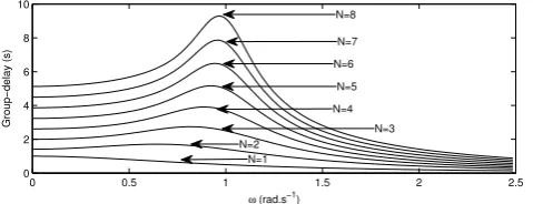
The group-delay of the integer Butterworth filter is the time needed for each frequency component of the filtered signal to pass through the filter and is defined as:
TBW(ω) =− N
X
k=1
ωccos π2+π2k2N−1
ω2
c −2ωcωsin π2 +π2k2−1N
+ω2
(14)
(a) Transport-delay filter. (b) Delayed fractional state variable filter.
Fig. 1: Gain, phase and transport-delay in (a) or group-delay in (b) of Γ(1jω), expressed in dashed, solid and dotted lines, respectively whereωc= 1 (rad.s−1).
0 0.5 1 1.5 2 2.5
0 2 4 6 8 10
ω (rad.s−1)
Group−delay (s)
N=4
N=3 N=5 N=6 N=7 N=8
[image:7.595.49.289.411.503.2]N=1 N=2
Fig. 2: Group-delay in (s) of the integer Butterworth filter, with orderN = 1 : 8 andωc= 1.
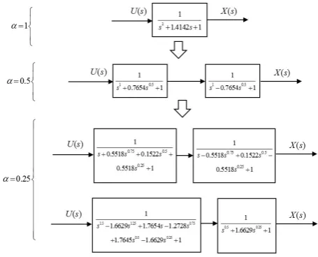
4.1.1 Square root base design (fractional Butterworth filter withα= 1
2n base-order)
This section demonstrates how the maximally flat gain frequency response of fractional Butterworth filter can be obtained with a restricted base-orderα= 1
2nwhere
n∈Z. There areN root terms in equation (12). When
α= 1 andN is an even number, the roots in equation (12) are given byN/2 complex pairs where ¯sk denotes the conjugate of sk. Each root term is considered to be a quadratic function, described by the difference of two squares (sand sk), and expressed in the standard quadratic form and factored form as:
s−sk
| {z }
Standard quadratic f orm
= s0.5−√sk
s0.5+√sk
| {z }
F actored quadratic f orm (15)
The factored quadratic form can be obtained by considering the square root of the complex number ac-cording to De Moivres theorem:
q √
sk = q
p
|sk|
cos
∠sk
q +
2πa q
+ sin
∠sk
q +
2πa q
(16)
wherea= 0,1 andNis assumed to be an even num-ber. From equation (15), it can be noted that each root term has two different complex roots√s=±√sk. The same techniques are applied to the root term which con-tains the complex conjugate ¯sk so that the two differ-ent conjugate roots±√s¯kare produced. For example, if
N = 2, the integer Butterworth denominator of equa-tion (12) is described as a product of two root terms as:
HB(s) = 1
s−−
√ 2
2 +j
√ 2
2 s−
−√2
2 j−
√ 2 2
(17)
The factored form of the root term which contains one complex root and the root term which contains the conjugate root can be obtained from equations (15) and (16), and presented as follows:
s−−√22 +j√22=
s0.5+ (0.38 +j0.92)
s0.5−(0.38 +j0.92)
s−−√2
2−j√2
2=
s0.5+ (0.38−j0.92)
s0.5−(0.38−j0.92)
(18)
The fractional Butterworth transfer function of half-base order, derived from equation (18), is expressed as:
HB(s) = 1
s0.5−0.38 +j0.92
s0.5−0.38−j0.92
(s0.5+ 0.38 +j0.92) (s0.5+ 0.38−j0.92)
(19)
However, in order to avoid returning to the integer-order Butterworth transfer function, the fractional But-terworth transfer function must be described by two subsystems as follows:
HB(s) =
1
(s−0.7654s0.5+ 1)
1
(s+ 0.7654s0.5+ 1)
(20)
From equation (16), all the fractional derivative terms can be obtained, which can then be used in the identi-fication process.
This can then be factored into eight root terms of base-order α = 0.25, and it is expressed as (21):
HB(s) =
1
s0.25−0.8315−j0.5556
s0.25−0.8315 +j0.5556
s0.25+ 0.5556−j0.8315
(s0.25+ 0.5556 +j0.8315) (s0.25+ 0.8315−j0.5556) (s0.25+ 0.8315 +j0.5556)
(s0.25−0.5556−j0.8315) (s0.25−0.5556 +j0.8315)
(21)
The N root terms of the integer Butterworth trans-fer function produce 2nN root terms of the fractional Butterworth filter of base-orderα= 1
2n. For example, the first order Butterworth transfer function generates 2 root terms of a fractional Butterworth filter of base-orderα= 0.5.
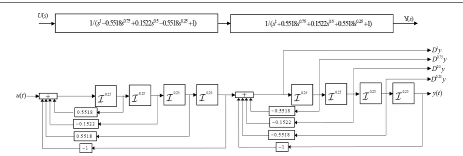
The Butterworth filter of base-order α = 0.25 in (21) can be described by two first-order subsystems (s1) or two subsystems whose orders are (s1.5) and (s1.5)
as shown in Fig 4 and, respectively, expressed as (22):
HB(s) = 1
s+ 0.0.5518s0.75+ 0.1522s0.5+ 0.5518s0.25+ 1
s−0.0.5518s0.75+ 0.1522s0.5−0.5518s0.25+ 1
= 1
(s1.25−1.6629s1.25+ 1.7654s−1.2728s0.75+ 1.7645s0.5−1.6629s0.25+ 1) s0.5+ 1.6629s0.25+ 1
(22)
The following algorithm can be used to directly gener-ate the roots of the denominator of the fractional But-terworth filter of base-orderα= 1
2n:
r= 0
fork= 1 :N
θ=π 1
2 + (2k−1)
2N
fora= 0 :m−1
r=r+ 1
s
12n
k = m
√ ωc
ej
θm+2απm
(23)
end end
where m= 2n,M =mN, a= 0,1,· · ·, m−1 and
k= 1,2,· · · , N .
because it is derived from a stable integer Butterworth filter.
Summary of the design
(i) Design the classical integer Butterworth filter. (ii) Obtain the factored quadratic form of each root
term of the integer Butterworth transfer function by using the complex square roots in (16) for gener-ating the root terms of the fractional Butterworth filter of base-orderα= 12 . The fractional Butter-worth filter of base-order α= 1
4 is then derived from the fractional Butterworth filter of base-order
α= 12. Likewise, the fractional Butterworth filter of base-orderα= 1
2pis then derived from the frac-tional Butterworth filter of base-order α= 1
2p−1
until the targeted base-order is obtained. Further-more, the roots of the denominator of the fractional Butterworth transfer function of the targeted base-order could be directly derived from the integer But-terworth transfer function by using (23).
4.1.2 Compartmental fractional Butterworth filter design
The proposed compartmental FBF is derived from the integer Butterworth filter which is simulated in Simulink using integer integral block, see [35]. Every integer in-tegral term is compartmentally divided into its equiva-lent fractional integral terms (If(t) =R0tf(t)dt), based on the semigroup property of fractional integral of the arbitrary order IαIβ = Iα+β, stated in [34]. Conse-quently, the integer integral block in equivalent block diagram form can be represented by a series of
[image:9.595.307.523.173.284.2]frac-Fig. 3: CFBF of base-order α = 0.5 and α = 0.25, derived from CIBF whereU(s) andX(s) are the input and output of Butterworth filter, respectively.
Fig. 4: A block diagram of the fractional integral block.
Fig. 5: Compartmental FBF of the first order for ap-proximating the fractional derivative termD0.7v(t).
tional integral blocks. This is additional to the prop-erty of fractional calculus which takes the fractional derivative term to be the right inverse of the fractional integral termIαDα=I, whereIdenotes the identity or unity. This property is valid only when considering zero initial conditions, see [34]. Thus, any fractional deriva-tive term can be obtained. This approach can be sum-marised by the following two steps:
(i) Exploiting the property that the inverse operator of the fractional integral term is the right inverse of the fractional integral term, when considering zero initial conditions. This allows obtaining any frac-tional derivative term from the fracfrac-tional integral as shown in Fig. 4.
(ii) The semigroup property of the fractional integral of arbitrary order allows splitting up an integer or-der integral into compartmental form to produce the targeted order.
For example, if there is a need to approximate an ar-bitrary α derivative term of the output signal v(t) of the Butterworth filter in Fig. 3, whose order isN = 1, the first order integral block can be split into, for ex-ample, α= 0.7 and β = 0.3 fractional integral blocks as shown in Fig. 5. Considering the semigroup property it is possible to see that a full integer order integration still takes place, i.e. I0.7I0.3 =I, hence the
[image:9.595.45.273.519.703.2]4.2 Group-delay equalisation: All-pass filter
The designed FBF has been derived based on the clas-sical integer Butterworth filter without changing its non-uniform group-delay. Therefore, it is proposed to adapt the all-pass filter for group-delay equalisation of the FBF, within a selected pass-band, resulting in the overall DFSVF. A second order transfer function of the all-pass filter is expressed as [8]:
HAP(s) =
(s−c)2+d2
(s+c)2+d2 (24)
where c >0 for generating a stable filter and the sub-script AP denotes all-pass filter. The group-delay of the second order all-pass filter is given by:
TAP(ω) =
4c(ω2+c2+d2)
(c2+d2−ω2)2+ 4c2ω2 (25)
The overall group-delay of DFSVF is then defined as the sum of the group-delays of all-pass filter and cascaded FBF, where this should equal to a constant, frequency independent, delay, denotedT0. According to
[8], the parameterscanddare then found by solving a following non-linear least squares problem:
=
Z ωT max 0
[T0−TBW(ω)−TAP(ω)]
2
(26)
where TAP(ω) and TBW(ω) are the frequency depen-dent group delays of the all-pass filter and the integer Butterworth filter defined in (25) and (12), respectively. The group delay equalisation is performed only in a pre-defined low frequency rangeω= 0 toω=ωT max, where atωT maxtheTBW(ω) reaches its maximum value.
When increasing the order of integer Butterworth filter the slope of group delayTBW(ω) (equivalent to the group delay of FBF) becomes more steep and uneven, within the frequency range of interest ω= (0, ωT max), see Fig. 2. Consequently, in order to equalise the group delayTBW(ω) higher order all-pass filter must be used. So far, the only single second order all-pass filter has been introduced in (24), where higher order all-pass fil-ter can be obtained by cascading several second order all-pass filters into stages. Consequently, as the order of the all-pass filter increases more individualc andd
parameters must be found.
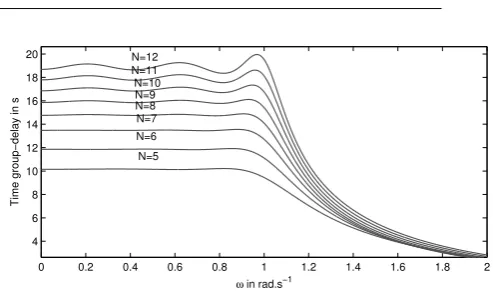
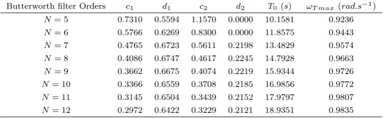
In order to assess the performance of the group delay equalisation two following examples are consid-ered. Firstly, a Butterworth filter with cut-off frequency
ωc = 1 (rad.s−1) and filter orders ranging fromN = 5 to N = 12 is considered. A two stage all-pass filter is selected, i.e. a cascade connection of two second order
HAP(s) filters. The number of stages is denoted M, whereM = 2 in this example. Table 1 shows the found
0 0.2 0.4 0.6 0.8 1 1.2 1.4 1.6 1.8 2 4
6 8 10 12 14 16 18 20
ω in rad.s−1
Time group−delay in s
N=12
N=10 N=11
N=9 N=8 N=7 N=6
[image:10.595.314.561.76.222.2]N=5
Fig. 6: Group delay of DFSVF with two stage all-pass filter and cut-off frequencyωc= 1 (rad.s−1). The order of Butterworth filter ranges fromN = 5 toN= 12.
0 5 10 15 20 25 30 0.5
1 1.5 2 2.5
ω (rad.s−1)
Group−delay (s)
9 Stages
7 Stages 5 Stages
3 Stages 1 Stage
No Stages
Fig. 7: Group delay of DFSVF with stages of all-pass filter ranging from M = 1 to M = 9. The order of Butterworth filter isN = 8 with cut-off frequencyωc= 12 (rad.s−1). The case when no all-pass filter is used is also shown, i.e. only the group delay of the Butterworth filter is plotted.
all-pass filter parameters for stageM = 1 andM = 2, which are denoted (c1, d1) and (c2, d2), respectively.
The table also shows the found approximated group delay T0 and ωT max. Corresponding Fig. 6 shows the
overall obtained group delay of the DFSVF, where the closer the order of the all-pass filter to the order of the Butterworth filter the better equalisation is achieved. This is especially true for ordersN = 5 andN = 6. In other words, selecting the number of the all-pass filter stages mainly depends on the Butterworth order.
Secondly, a Butterworth filter with cut-off frequency
ωc = 12 (rad.s−1) and a fixed order N = 8 is chosen. All-pass filter stages range from M = 1 to M = 9 are shown in 7. Table 2 shows the found all-pass filter parameters for all stages as well as the approximated delay T0. In general, the higher the number of stages
[image:10.595.312.527.298.408.2]Table 1: Parameters of two stage all-pass filter when equalizing a Butterworth filter with cut-off frequencyωc = 1 (rad.s−1) and orders ranging fromN = 5 toN = 12.
Butterworth filter Orders c1 d1 c2 d2 T0(s) ωT max(rad.s−1)
N= 5 0.7310 0.5594 1.1570 0.0000 10.1581 0.9236
N= 6 0.5766 0.6269 0.8300 0.0000 11.8575 0.9443
N= 7 0.4765 0.6723 0.5611 0.2198 13.4829 0.9574
N= 8 0.4086 0.6747 0.4617 0.2245 14.7928 0.9663
N= 9 0.3662 0.6675 0.4074 0.2219 15.9344 0.9726
N= 10 0.3366 0.6559 0.3708 0.2185 16.9856 0.9772
N= 11 0.3145 0.6504 0.3439 0.2152 17.9797 0.9807
[image:11.595.89.491.288.435.2]N= 12 0.2972 0.6422 0.3229 0.2121 18.9351 0.9835
Table 2: All-pass filter parameters for stages ranging fromM = 1 toM = 9. Butterworth filter cut-off frequency isωc = 12 (rad.s−1) and orderN = 8.
T0 i M= 1 M= 2 M= 3 M= 4 M= 5 M= 6 M= 7 M= 8 M= 9
0.8819 ci 5.6700 − − − − − − − −
di 4.5222 − − − − − − − −
1.3769 ci 8.9502 8.9500 8.9504 − − − − − −
di 5.8805 5.8806 5.8806 − − − − − −
1.7856 ci 10.698 10.698 10.698 10.698 10.698 − − − −
di 6.6533 6.6533 6.6534 6.6533 6.6533 − − − −
2.0622 ci 18.087 13.377 20.439 15.491 17.316 17.140 5.8819 − −
di 0.8265 2.7210 1.1312 1.4624 0.8546 0.8785 8.6657 − −
2.3167 ci 19.450 19.870 19.484 19.557 20.317 19.572 21.230 14.687 5.9750
di 0.4351 0.6444 0.4578 0.4910 0.8413 0.5015 1.1094 0.1490 8.7329
5 DFSVF implementation and estimation process
The implementation and simulation of the delayed state variable filter are essential steps to proper parameter es-timation. The system of equation defined in the state space representation or a transfer function can be ex-pressed in an equivalent block diagram as a state vari-able filter and more information can be found in [36, 2]. The equivalent block diagram allows collecting the derivatives of the signals in clearer and easier manner by implementing it in Simulink. It is then numerically solved at each sample by using one of the Simulink solvers such as the Euler or Runge-Kutta solver.
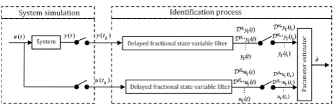
In previous sections, FBF and all-pass filter are indi-vidually treated. However, all these filters can be com-bined in one filter called delayed fractional state vari-able filter for generating delayed fractional derivative terms whether they are linear or nonlinear. Thus, the delayed state variable filter is simulated in two steps as illustrated in Fig. 8. The all-pass filters are firstly and individually cascaded and simulated in Simulink.
The output of the cascaded all-pass filters is used as an input to simulate the fractional Butterworth filter
in Simulink. From fractional Butterworth filter, all the higher fractional derivative terms of the filtered signals can be obtained. For instance, an arbitrary signaly(t) is passed through the delayed fractional state variable filter. Consequently, the filtered or delayedy(t) is pro-duced and denoted yΓ(t). Furthermore, all the higher fractional derivative terms Dαiy
Γ(t)(t) =
dαiyΓ(t)(t)
dtαi
can be collected from fractional Butterworth.
Fig. 8 demonstrates the input and the outputs of the delayed fractional state variable filter where in later sec-tions the input will be the signals, which are collected for identification. The system simulation and identifi-cation process steps are illustrated in Fig. 9.
6 Simulation study
Fig. 8: Block Diagram of the delayed state variable filter simulation.
Fig. 9: System simulation and identification process.
6.1 Comparison of the proposed approaches
Two approaches for designing the fractional-order But-terworth filter has been proposed in this paper, namely, the square root base design and compartmental fractional-order Butterworth filter design.
The comparison made in this section is used to sup-port the selection of one approach to be used in approx-imating the higher fractional-order derivative terms of the output of the Butterworth filter in the numeri-cal example that will foloow. Accordingly, in this sec-tion, an illustrative example is used as a benchmark to evaluate the performance of the two proposed ap-proaches. The second order classical Butterworth filter is used as a reference to validate both approaches and is also used to approximate the higher fractional-order derivative terms. For instance, if we take the Butter-worth output v(t) andD0.25v(t) are the collected
tar-gets. The square root base fractional Butterworth filter (SRBFBF) is second order and is shown in Fig. 10. It can be observed that this approach has eight fractional-order integral blocks. This requires computational time compared to the compartmental fractional Butterworth filter (CFBF) which only has three fractional-order in-tegral blocks, as illustrated in Fig. 11. The simulation
runs for 5 s by using Simulink and MATLABR. The solver is selected to be Runge-Kutta with 0.001s sam-pling time. Fractional-order integral blocks are from The FOMCON Simulink block library where approx-imation order and frequency range are set to fifth or-der and [0.001; 100] rad.s−1, respectively. The input is selected as a sum of the sinusoid signals within the range of the fractional-order integral blocks range as il-lustrated in Fig. 12. The integral of the absolute error (IAE) between the output and higher fractional-order derivative terms, obtained from the integer-order But-terworth filter, are compared with those obtained by the CFBF and SRBFBF.
The Butterworth filter output, theDv(t) terms based on the three different designs and the D0.25v(t) terms
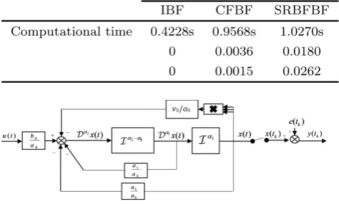
of both fractional-order filter designs are shown in Figs. 13, 14, and Table 3. It can readily be seen from Table 3 that the CFBF provides a better approximation to the reference filter, i.e. the classical Butterworth filter, as compared to the SRBFBF in terms of IAE measure. This improved filtering performance of CFBF is further visible in Figs. 13, 14, where the filtered signals are seen to be closer to their reference counterpart. The error that is present is the numerical error associated with each fractional-order integral block. This error scales with the number of fractional-order integral blocks used and consequently more pronounced for the SRBFBF. The results, obtained from 13, and Table 3, favour se-lection of the compartmental approach over the square root approach. It is noteworthy to highlight that:
(I) The design process of the compartmental approach is considerably simpler than the square root based approach.
(II) The compartmental approach can be applied to ob-tain any fractional-order, which is not the same with the square root based approach that is limited by base-order α=1/2n.
(III) A higher numerical accuracy is achieved using the compartmental approach relative to the square root based approach for approximation of the same fractional-order derivative term.
(IV) The computational time of the compartmental ap-proach is relatively smaller than the computational time of the square root approach.
(V) The compartmental approach presented better ca-pability in generating any arbitrary fractional-order derivative terms.
This leads to the compartmental approach being the favourable method; adopting this method also increases the adaptability to non-commensurate systems.
[image:12.595.41.281.314.392.2]Fig. 10: The upper part shows the transfer function of the two subsystems representing fractional-order-Butterworth filter and the equivalent block diagram by applying square root base for base-orderα= 1/2 where
[image:13.595.301.548.304.431.2]α= 1/4 andωc = 1.
[image:13.595.43.302.307.402.2]Fig. 11: Second order fractional-order Butterworth filter using compartmental approach whereωc= 1.
Fig. 12: Input is used for simulation.
how to extend the approximated integer Butterworth filter to an FBF. For example, Soltan, Rawan and Soli-man [41] have extended a two element integer But-terworth filter to fractional-order in the case of the commensurate order and higher commensurate orders, see [1]. In their work, similar coefficients of a classi-cal integer Butterworth filter are used for FBF. This filter was been further extended to have two different non-equal base-orders for non-commensurate orders in [42]. This is achieved by first transforming the FBF to the frequency-domain. The generated nonlinear equa-tion is then optimised to obtain the best flat gain, with consideration given to stability. However, these are no
Fig. 13: Bold grey solid-line is the integer-order But-terworth filter output v(t), black doted-line and black dashed-line represent the CFBF output v(t) and the SRBFBF outputv(t), respectively.
Fig. 14: Bold grey solid-line is the derivative term
Dv(t) of the integer-order Butterworth filter and black doted-line and black dashed-line represent the deriva-tive termsDv(t) of CFBF and SRBFBF, respectively.
[image:13.595.47.298.450.548.2] [image:13.595.298.548.501.630.2]Table 3: The calculated IAE performance measure to-gether with corresponding frequency ranges for different integer model orders of approximated fractional mod-els.
IBF CFBF SRBFBF
Computational time 0.4228s 0.9568s 1.0270s 0 0.0036 0.0180
0 0.0015 0.0262
Fig. 15: The equivalent block diagram of (27) with con-sidering noise.
equivalent circuit model is used, where it is relatively easy to adapt fractional-order theory, but this approach becomes increasingly more complex as the number of elements increase.
6.2 Numerical example
The performance of the presented delayed fractional state variable identification approach is demonstrated on a parameter estimation problem of fractional non-linear Duffing’s oscillator [36]. The system model is de-scribed by a following ordinary fractional nonlinear dif-ferential equation:
S
(
a0Dα2x(t) +a1Dα1x(t) +a
2x(t) +v0x3(t) =b0u(t) y(tk) =x(tk) +e(tk)
(27)
where the measured output is corrupted by additive, white, zero mean noise with Gaussian distribution with variance σe2. The noise variance is selected such that a prescribed signal to noise ratio, denoted SN R, is achieved. TheSN R is defined indB by 10 log(σ2
x/σe2), whereσx2denotes the variance of noise free system out-putx(t). The model parameters are chosen to be:a0=
1, a1 = 1, v0 = 0.6, b0 = 1 and parameter a2 is
nor-malised to unity. Two fractional order cases are consid-ered, firstly, commensurate with α1 = 0.5 and α2 = 1
and, secondly, non-commensurate fractional order with
α1= 0.7 andα2= 1.
The system in (27) can be simulated in Simulink by using equivalent block diagram as shown in Fig. 15.
The input signal is selected to be a sum of 10 sinu-soids whose bandwidth isω= 1 (rad.s−1). The highest frequency of system, required to be covered is approx-imately 3-5 times the bandwidth of the input signals. This is because for low pass characteristics and systems having mild nonlinearities, the response of the system output can be well tackled by the first 3-5 Volterra ker-nels [50].
This simulation has been run over a time period of 50 (s) with a simulation time step of Ts = 0.001 (s). The selected Simulink solver is ode4 (Runge-Kutta). The Simulink fractional integral block-set, required to implement FBF, is provided by FOMCON Simulink li-brary with the following setting: The interesting fre-quency range of the fractional integral term has been selected to be [0.001,1000] (rad.s−1) in order to guar-antee the noise in high frequencies is not filtered by the integral approximation. The FOMCON library uses the modified Oustaloup method and the coefficient selec-tion is connected more to the numerical study require-ments but not connected with the DFSVF implemen-tation. There are more numerical methods for approx-imating the fractional integral terms such as Carlson’s and Matsuda’s methods [38]. The DFSVF has been de-signed with eighth order FBF, N = 8, and cut-off fre-quency of ωc = 12 (rad.s−1). Nine stages of the sec-ond order all-pass filter,M = 9, are chosen to achieve approximately constant group-delay. The bandwidth of the Butterworth filter is selected to handle the entire output range of frequencies.
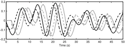
Figs. 16a, 16b and 17 show the performance of the selected commensurate DFSVF applied to system input and output signals, respectively, with SN R = 20dB. For example, considering Fig. 16a, the filtered input signal (solid black line) is delayed approximately by 2.3 (s), while only little to no shape distortion is cased by the filtering process, as expected. Furthermore, the noise in the filtered output has been significantly re-duced as shown Fig. 16b because the DFSVF performs as a low pass filter. Fig. 17 shows the noise-free frac-tional signal derivativesD0.5x(t) (solid black line) and Dx(t) (dashed black line) and their corresponding fil-tered measured counterpartsD0.5y(t) (solid grey line),
andDy(t) (dashed grey line), respectively. A small shape distortion of the filtered derivative signals is visible in Fig. 17 due to relatively high signal to noise ratio, as expected, indicating a high performance of the designed DFSVF.
0 5 10 15 20 25 30 35 40 45 50 −0.5
0 0.5
Time (s)
(a)
0 5 10 15 20 25 30 35 40 45 50
−0.4 −0.2 0 0.2 0.4
Time (s)
[image:15.595.45.264.72.272.2](b)
Fig. 16: Subplot (a) shows sampled input signal u(t) (solid grey line) and filtered input uΓ(t) (solid black line). Subplot (b) shows noise-free outputx(t) (dashed black line), measured noisy output y(t) (solid grey line), and filtered noisy output yΓ(t) (dashed black line). Commensurate system order is considered for
SN R= 20dB.
0 5 10 15 20 25 30 35 40 45 50
−0.2 −0.1 0 0.1 0.2
Time (s)
Fig. 17: Noise-free fractional signal derivativesD0.5x(t)
(solid black line) and Dx(t) (dashed black line) with their corresponding filtered measured counterparts
D0.5y(t) (solid grey line) andDy(t) (dashed grey line).
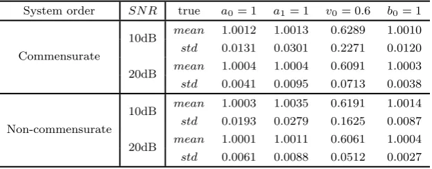
standard deviations of parameter estimates are pre-sented for comparing the statistical efficiency of the proposed identification approach. Two different noise strengths scenarios are evaluated with lowSN R= 10dB
and highSN R= 20dB. The obtained results indicate a high parameter estimation accuracy for both the com-mensurate and non-comcom-mensurate system orders de-spite the presence of significant measurement noise.
7 Conclusions
The delayed fractional state variable identification ap-proach for parameter estimation of a class of fractional nonlinear ordinary differential equation models, in the continuous-time domain, has been presented. The core part of this approach comprises of the proposed
de-layed fractional state variable filter (DFSVF) in a con-nection with a suitable parameter estimation method. The DFSVF contains a cascade of all-pass filters, for group delay equalisation, and proposed, a novel, frac-tional Butterworth filter (FBF).
The comparison study illustrates that the compart-mental fractional Butterworth filter (CFBF) showed better performance in the delayed fractional state vari-able identification approach over the square root base fractional Butterworth (SRBFB) of in terms of gener-ality (the proposed CFBF can generate any arbitrary fractional terms while SRBFB is limited with base-orderα=1/
2n), simplicity and computational accuracy
and computational time. However, both approaches and FBF offer the following advantages: i) they are simpler in derivation because they are built on the well-known integer Butterworth filter. The extra step is to use well-known properties of the integral and avoiding the use of optimisation algorithms or square roots of complex terms; iii) the performance of the proposed FBF gen-erates and guarantees maximum flat gain because it holds the properties of the integer Butterworth filter; and iv) the proposed compartmental and square root base approaches can be mapped to extend any other linear filter directly from the classical integer linear fil-ter.
The required property of the DFSVF is to have a maximally flat magnitude response and constant group delay in a selected frequency band in order to achieve the required commutative property for subsequent model parameter estimation. It has been revealed that the or-der of all-pass filter depends on the oror-der of fractional Butterworth filter and the selected cut-off frequency of DFSVF.
The presented delayed fractional state variable iden-tification approach is demonstrated on a parameter es-timation problem of fractional nonlinear Duffings os-cillator and its performance has been assessed via a Monte-Carlo simulation study. The measured, sampled, input-output data were used to show the practicality of the proposed method. A consistent performance has been achieved for various noise strength scenarios with small standard deviations of parameter estimates.
[image:15.595.56.268.386.467.2]Table 4: Monte Carlo simulation results for fractional-order continuous-time nonlinear commensurate (α1 =
0.5, α2= 1) and non-commensurate (α1= 0.7, α2= 1) system.
System order SN R true a0= 1 a1= 1 v0= 0.6 b0= 1
Commensurate
10dB mean 1.0012 1.0013 0.6289 1.0010
std 0.0131 0.0301 0.2271 0.0120
20dB mean 1.0004 1.0004 0.6091 1.0003
std 0.0041 0.0095 0.0713 0.0038
Non-commensurate
10dB mean 1.0003 1.0035 0.6191 1.0014
std 0.0193 0.0279 0.1625 0.0087
20dB mean 1.0001 1.0011 0.6061 1.0004
std 0.0061 0.0088 0.0512 0.0027
on-line application. This extends the applicability of the proposed approach to fields of model based systems monitoring, fault detection, adaptive observer design, and adaptive control.
For further work, the proposed approach will be compared with other approaches such as the optimisa-tion based approaches to highlight strengths and weak-nesses in light of different noise processes.
Conflicts of interest: All authors declare that they have no conflict of interest.
References
1. Acharya, A., Das, S., Pan, I., Das, S.: Extending the con-cept of analog butterworth filter for fractional order sys-tems. Signal Processing94, 409–420 (2014)
2. Allafi, W., Burnham, K.J.: Identification of fractional-order continuous-time hybrid box-jenkins models using refined instrumental variable continuous-time fractional-order method. In: Advances in Systems Science - Pro-ceedings of the International Conference on Systems Sci-ence, pp. 785–794 (2013)
3. Allafi, W., Uddin, K., Zhang, C., Sha, R.M.R.A., Marco, J.: On-line scheme for parameter estimation of nonlinear lithium ion battery equivalent circuit mod-els using the simplified refined instrumental variable method for a modified wiener continuous-time model. Applied Energy 204, 497 – 508 (2017). DOI http://dx.doi.org/10.1016/j.apenergy.2017.07.030 4. Allafi, W., Zajic, I., Burnham, K.J.: Identification of
Fractional Order Models: Application to 1D Solid Dif-fusion System Model of Lithium Ion Cell, pp. 63–68. Springer International Publishing, Cham (2015) 5. Anderson, S.R., Kadirkamanathan, V.: Modelling and
identification of non-linear deterministic systems in the delta-domain. Automatica43(11), 1859–1868 (2007) 6. Aslam, M.S., Chaudhary, N.I., Raja, M.A.Z.: A
sliding-window approximation-based fractional adaptive strat-egy for hammerstein nonlinear armax systems. Nonlinear Dynamics87(1), 519–533 (2017). DOI 10.1007/s11071-016-3058-9
7. Azar, A., Vaidyanathan, S., Ouannas, A.: Fractional or-der control and synchronization of chaotic systems, vol. 688. Springer (2017)
8. Blinchikoff, H.J.: Filtering in the Time and Frequency Domains. Electromagnetic Waves. Institution of Engi-neering and Technology (2001)
9. Buller, S., Thele, M., Karden, E., Doncker, R.W.D.: Impedance-based non-linear dynamic battery mod-eling for automotive applications. Journal of Power Sources 113(2), 422 – 430 (2003). DOI https://doi.org/10.1016/S0378-7753(02)00558-X. Pro-ceedings of the International Conference on Lead-Acid Batteries,{LABAT}’02
10. Butterworth, S.: On the theory of filter amplifiers. Wire-less Engineer7(6), 536–541 (1930)
11. Cahoy, D.O., Uchaikin, V.V., Woyczynski, W.A.: Parameter estimation for fractional poisson pro-cesses. Journal of Statistical Planning and In-ference 140(11), 3106 – 3120 (2010). DOI http://dx.doi.org/10.1016/j.jspi.2010.04.016
12. Chen, D., Chen, Y., Xue, D.: Digital fractional order savitzky-golay differentiator. IEEE Transactions on Cir-cuits and Systems II: Express Briefs 58(11), 758–762 (2011). DOI 10.1109/TCSII.2011.2168022
13. Chen, Y., Wei, Y., Zhou, X., Wang, Y.: Stabil-ity for nonlinear fractional order systems: an indi-rect approach. Nonlinear Dynamics 89(2), 1011– 1018 (2017). DOI 10.1007/s11071-017-3497-y. URL https://doi.org/10.1007/s11071-017-3497-y
14. Cois, O., Oustaloup, A., Poinot, T., Battaglia, J.L.: Frac-tional state variable filter for system identification by fractional model. In: 2001 European Control Conference (ECC), pp. 2481–2486 (2001)
15. Essa, M., Aboelela, M., Hassan, M.: Application of frac-tional order controllers on experimental and simulation model of hydraulic servo system. In: Fractional Order Control and Synchronization of Chaotic Systems, pp. 277–324. Springer (2017)
16. Garnier, H., Wang, L., Young, P.C.: Direct Identification of Continuous-time Models from Sampled Data: Issues, Basic Solutions and Relevance, pp. 1–29. Springer Lon-don, London (2008)
17. Guti´errez, R.E., Ros´ario, J.M., Tenreiro Machado, J.: Fractional order calculus: basic concepts and engineer-ing applications. Mathematical Problems in Engineerengineer-ing
2010(2010)
18. Hartley, T.T., Lorenzo, C.F., Qammer, H.K.: Chaos in a fractional order chua’s system. IEEE Transactions on Circuits and Systems I: Fundamental Theory and Appli-cations42(8), 485–490 (1995). DOI 10.1109/81.404062 19. Hilfer, R.: Applications of fractional calculus in physics.
20. Karami-Mollaee, A., Tirandaz, H., Barambones, O.: On dynamic sliding mode control of nonlinear fractional-order systems using sliding observer. Nonlinear Dynamics
92(3), 1379–1393 (2018). DOI 10.1007/s11071-018-4133-1. URL https://doi.org/10.1007/s11071-018-4133-1 21. Khadhraoui, A., Jelassi, K., Trigeassou, J.C., Melchior,
P.: Identification of fractional model by least-squares method and instrumental variable. Journal of Compu-tational and Nonlinear Dynamics 10(5), 050801–01–10 (2015)
22. Kohr, R.H.: A method for the determination of a dif-ferential equation model for simple nonlinear systems. Electronic Computers, IEEE Transactions onEC-12(4), 394–400 (1963)
23. Leyden, K., Goodwine, B.: Fractional-order system iden-tification for health monitoring. Nonlinear Dynamics
92(3), 1317–1334 (2018). DOI 10.1007/s11071-018-4128-y. URL https://doi.org/10.1007/s11071-018-4128-y 24. Li, Z., Chen, D., Zhu, J., Liu, Y.: Nonlinear
dynam-ics of fractional order duffing system. Chaos, Solitons & Fractals 81, Part A, 111 – 116 (2015). DOI https://doi.org/10.1016/j.chaos.2015.09.012
25. Lin, J., Wang, Z.J.: Parameter identification for fractional-order chaotic systems using a hybrid stochas-tic fractal search algorithm. Nonlinear Dynamics90(2), 1243–1255 (2017). DOI 10.1007/s11071-017-3723-7. URL https://doi.org/10.1007/s11071-017-3723-7
26. Liu, D.Y., Gibaru, O., Perruquetti, W., Laleg-Kirati, T.M.: Fractional order differentiation by integration and error analysis in noisy environment. IEEE Transactions on Automatic Control60(11), 2945–2960 (2015). DOI 10.1109/TAC.2015.2417852
27. Liu, D.Y., Laleg-Kirati, T.M., Gibaru, O., Perruquetti, W.: Fractional Order Numerical Differentiation with B-Spline Functions. In: The International Conference on Fractional Signals and Systems 2013. Ghent, Belgium (2013)
28. Liu, D.Y., Zheng, G., Boutat, D., Liu, H.R.: Non-asymptotic fractional order differentia-tor for a class of fractional order linear sys-tems. Automatica 78, 61 – 71 (2017). DOI http://dx.doi.org/10.1016/j.automatica.2016.12.017 29. Liu, F., Li, X., Liu, X., Tang, Y.: Parameter
identifica-tion of fracidentifica-tional-order chaotic system with time delay via multi-selection differential evolution. Systems Science & Control Engineering5(1), 42–48 (2017)
30. Maachou, A., Malti, R., Melchior, P., Battaglia, J.L., Hay, B.: Thermal system identification using fractional models for high temperature levels around different operating points. Nonlinear Dynamics 70(2), 941– 950 (2012). DOI 10.1007/s11071-012-0507-y. URL https://doi.org/10.1007/s11071-012-0507-y
31. Maachou, A., Malti, R., Melchior, P., Battaglia, J.L., Oustaloup, A., Hay, B.: Nonlinear thermal system iden-tification using fractional volterra series. Control Engi-neering Practice29, 50 – 60 (2014)
32. Malti, R., Sabatier, J., Ak¸cay, H.: Thermal modeling and identification of an aluminum rod using fractional cal-culus. IFAC Proceedings Volumes 42(10), 958 – 963 (2009). DOI https://doi.org/10.3182/20090706-3-FR-2004.00159. 15th IFAC Symposium on System Identi-fication
33. Mani, A.K., Narayanan, M.D., Sen, M.: Parametric iden-tification of fractional-order nonlinear systems. Nonlinear Dynamics (2018). DOI 10.1007/s11071-018-4238-6. URL https://doi.org/10.1007/s11071-018-4238-6
34. Monje, C.A., Chen, Y., Vinagre, B.M., Xue, D., Feliu-Batlle, V.: Fractional-order systems and controls: funda-mentals and applications. Springer Science & Business Media (2010)
35. Nise, N.: Control systems engineeringl, 6 edn. Wiley (2011)
36. Petras, I.: Fractional-order nonlinear systems: modeling, analysis and simulation. Springer Science & Business Media (2011)
37. Raja, M., Chaudhary, N.: Adaptive strategies for param-eter estimation of box-jenkins systems. IET Signal Pro-cessing8, 968–980(12) (2014)
38. Sheng, H., Chen, Y., Qiu, T.: Fractional processes and fractional-order signal processing: techniques and appli-cations. Springer-Verlag London Springer (2012) 39. Sierociuk, D., Dzielinski, A.: Fractional kalman filter
al-gorithm for the states, parameters and order of fractional system estimation. International Journal of Applied Mathematics and Computer Science16(1), 129 (2006) 40. Simpkins, A.: System identification: Theory for the user,
2nd edition (ljung, l.; 1999) [on the shelf]. IEEE Robotics Automation Magazine 19(2), 95–96 (2012). DOI 10.1109/MRA.2012.2192817
41. Soltan, A., Radwan, A., Soliman, A.M.: Butterworth pas-sive filter in the fractional-order. In: International Con-ference on Microelectronics, pp. 1–5. IEEE (2011) 42. Soltan, A., Radwan, A., Soliman, A.M.: Fractional order
filter with two fractional elements of dependant orders. Microelectronics Journal43(11), 818–827 (2012) 43. Tang, Y., Zhang, X., Hua, C., Li, L., Yang, Y.:
Pa-rameter identification of commensurate fractional-order chaotic system via differential evolution. Physics Letters A376(4), 457 – 464 (2012)
44. Tepljakov, A., Petlenkov, E., Belikov, J.: Fomcon: Fractional-order modeling and control toolbox for mat-lab. In: Proceedings of the 18th International Conference Mixed Design of Integrated Circuits and Systems -MIXDES 2011, pp. 684–689 (2011)
45. Tsang, K., Billings, S.: Identification of continuous time nonlinear systems using delayed state variable filters. In-ternational Journal of Control60(2), 159–180 (1994) 46. Verhulst, F.: Nonlinear differential equations and
dynam-ical systems. Springer Science & Business Media (2006) 47. Victor, S., Malti, R., Garnier, H., Oustaloup, A.:
Pa-rameter and differentiation order estimation in fractional models. Automatica 49(4), 926 – 935 (2013). DOI http://dx.doi.org/10.1016/j.automatica.2013.01.026 48. Wang, L., Gawthrop, P.: On the estimation of continuous
time transfer functions. International Journal of Control
74(9), 889–904 (2001). DOI 10.1080/00207170110037894 49. Welty, J.R., Wicks, C.E., Rorrer, G., Wilson, R.E.: Fun-damentals of momentum, heat, and mass transfer. John Wiley & Sons (2009)
50. Wiener, D., SPINA, J.: Sinusoidal Analysis and Mod-elling of weakly Non-linear Circuits. New York: Van Nos-trand Reinhold (1980)
51. Winder, S.: Analog and digital filter design. Newnes (2002)
52. Young, P.C.: Recursive estimation and time-series anal-ysis: An introduction for the student and practitioner. Springer Science & Business Media (2011)