Exploring the Sensitivity of Coastal Inundation Modelling to DEM
Vertical Error
Harry West, Michael Horswell & Nevil Quinn
Abstract
As sea level is projected to rise throughout the 21st century due to climate change, there is a need to ensure that sea level rise (SLR) models accurately and
defensibly represent future flood inundation levels to allow for effective coastal
zone management. Digital Elevation Models (DEMs) are integral to SLR
modelling, but are subject to error, including in their vertical resolution. Error in
DEMs leads to uncertainty in the output of SLR inundation models, which if not
considered, may result in poor coastal management decisions. However, DEM
error is not usually described in detail by DEM suppliers; commonly only the
RMSE is reported. This research explores the impact of stated vertical error in
delineating zones of inundation in two locations along the Devon, United
Kingdom, coastline (Exe and Otter Estuaries). We explore the consequences of
needing to make assumptions about the distribution of error in the absence of
detailed error data using a 1m, publically available composite DEM with a
maximum RMSE of 0.15m, typical of recent LiDAR-derived DEMs. We
compare uncertainty using two methods (i) the NOAA inundation uncertainty
mapping method which assumes a normal distribution of error, and (ii) a
hydrologically correct bathtub method where the DEM is uniformly perturbed
between the upper and lower bounds of a 95% linear error in 500 Monte Carlo
Simulations (HBM+MCS). The NOAA method produced a broader zone of
uncertainty (an increase of 134.9% on the HBM+MCS method), which is
particularly evident in the flatter topography of the upper estuaries. The
HBM+MCS method generates a narrower band of uncertainty for these flatter
areas, but very similar extents where shorelines are steeper. The differences in
inundation extents produced by the methods relates to a number of underpinning
assumptions, and particularly, how the stated RMSE is interpreted and used to
represent error in a practical sense. Unlike the NOAA method, the HBM+MCS
model is computationally intensive, depending on the areas under consideration
and the number of iterations. We therefore used the HBM+ MCS method to
derive a regression relationship between elevation and inundation probability for
the Exe Estuary. We then apply this to the adjacent Otter Estuary and show that it
computationally intensive step of the HBM+MCS. The equation-derived zone of
uncertainty was 112.1% larger than the HBM+MCS method, compared to the
NOAA method which produced an uncertain area 423.9% larger. Each approach
has advantages and disadvantages and requires value judgements to be made.
Their use underscores the need for transparency in assumptions and
communications of outputs. We urge DEM publishers to move beyond provision
of a generalised RMSE and provide more detailed estimates of spatial error and
complete metadata, including locations of ground control points and associated
land cover.
Keywords: Sea Level Rise; DEM Error; Uncertainty; Digital Elevation or Terrain
Models; Coastal Applications
Introduction
Climate change induced sea level rise (SLR) is one of the most significant challenges facing the world’s coastal zone. An estimated 270 million people are at risk of a 1 in 100-year coastal flood event, a figure which is set to rise to 350 million by 2050 (Jongman et al., 2012). Sea level has been rising throughout the 20th century and between 1870 and 2004 global mean sea level rose 0.2m (Church and White, 2006). Under all SLR scenarios the frequency and magnitude of coastal flooding is likely to increase. In the UK, the 2009 UK Climate Projections (UKCP09) scenarios forecast a maximum SLR of 1.45m, and a minimum of 0.21m by 2100 (Sayers et al., 2015). For effective coastal zone management, it is important to identify the areas at risk of flooding from future SLR.
(French & Burningham, 2013), topography is a principal driver in many coastal change processes (Zhang, 2010).
Digital Elevation Models (DEMs), which represent topography, store elevation data on a cell-by-cell basis. However, all spatial datasets, including DEMs, have inherent inaccuracies introduced by errors from several sources, which propagate into uncertainty when used as data products (Fisher & Tate, 2006; Wechsler, 2007; Cooper & Chen, 2013). Understanding error and associated uncertainty, and how to
communicate and analyse these concerns, has been a significant challenge for the research community (Goodchild, 2010; Wallentin & Car, 2013). Discussions of uncertainty have moved from a simple acknowledgement, to being a key factor in GIS based decision-making (Couclelis, 2003; Tucci & Giordano, 2011). Decisions made using GIS data without consideration of uncertainty, may well be based on inaccurate and misleading understandings of spatial processes. This has the potential to affect the appropriateness of management and policy (Boin & Hunter, 2007). This is particularly problematic when mapping SLR (Rahmstorf, 2007), as although it is relatively simple to raise the water level on a DEM (Gesch, 2013), the accuracy and resolution with which the topography was originally mapped will affect the reliability of the results and model outputs (Coveney & Fotheringham, 2011; van de Sande et al., 2012).
both the vertical (RMSEz) and horizontal dimensions (RMSExy). Both represent the deviation of a modelled value from the true ground elevation/location (Gesch, 2013). Light Detection and Ranging (LiDAR) is a method of generating highly accurate DEMs. Recently large volumes of high quality LiDAR derived DEMs have become available. These are strongly suited to SLR assessments (Bales et al., 2007; Zhang, 2010) due to their low vertical error (Gesch, 2009). For example, some very high-resolution LiDAR derived DEMs (<50cm spatial high-resolution) have an RMSEz of 5cm. This is a significant improvement on DEMs derived using alternative methods, where the vertical error can exceed 2m (Poulter & Halpin, 2008). Earlier SLR assessments were based on such coarse scale DEMs (Poulter & Halpin, 2008; Li et al., 2009). However DEMs with high vertical errors have been found to be problematic for SLR assessment, and any results generated should be interpreted with caution (Santillan & Makinano-Santillan, 2017).
It is important to note that improvements in data quality do not necessarily remove the issue of error and associated uncertainty (Daly, 2006). Therefore as more high resolution products become freely available, exaggerated expectations of realism and accuracy need to be managed (Dottori et al., 2013) to avoid what Beven et al. (2015) refer to as ‘hyper-resolution ignorance’. Error and the resulting uncertainty of perceived higher quality products should be considered and understood for effective policy and management decision making.
Environment Agency released its LiDAR derived DEMs as open, freely downloadable data (at resolutions of 25cm, 50cm, 1m, and 2m). As these high resolution DEMs are more likely to be used in SLR assessments (Cooper & Chen, 2013), it is important to now consider the impact of their vertical error on the results of commonly used SLR models.
The paucity of research examining the impact of DEM vertical error on inundation extent arises for several reasons. Firstly, there is usually very limited information about error beyond the RMSE, and secondly there is little guidance as to what practitioners should assume this error measure represents, or indeed how it should be used to understand its consequence for coastal planning and decision making.
Finally, this may also be a result of the computationally intensive assessment process needed to present a defensible representation of resulting uncertainty. We aim to address this by assessing, quantifying, and presenting the uncertainty that arises in inundation due to stated vertical error within a publically available LiDAR-derived DEM using two different approaches. One of which makes the assumption of vertical errors being normally distributed at a point and across the DEM surface, while the other assumes a spatially random distribution of error, but drawn uniformly from between the upper and lower bounds of the 95% linear error. We will then explore the feasibility of developing elevation/uncertainty relationships based on one of these methods, and assess whether these relationships are adequately representative to replace intensive iterative approaches as an initial tool in assessing inundation extent and uncertainty associated with SLR projections.
Methodology
The UK Environment Agency’s 1m resolution LiDAR derived DEM was chosen
the study area. The DEM was projected according to the OSGB’36 British National Grid, with elevations recorded Above Ordnance Datum Newlyn (AODN). This DEM is a publically available composite data output. It is the product of 47 individual LiDAR surveys with varying RMSE values and systematic and random errors (available in the online supplementary material for this paper). No further data quality information was available for the either the composite data product or the individual surveys, as is the case with many similar datasets (Gesch, 2013). This includes precise details on the location of the ground control points (GCPs) and their associated landcover, or any further information regarding the spatial structure of the reported error across the composite DEM. As error will vary across the individual surveys, the quality control standards for the composite DEM will be used as model inputs in this research. The specifications for the DEM require horizontal (planar) accuracy, or absolute spatial error, of less than ±40cm (horizontal RSMExy=0.40m) (Environment Agency, 2016). For the 1m resolution DEM, this horizontal error is within the cell size and will therefore not be considered further. The vertical accuracy, or absolute height error, is required to be within ±15cm (vertical RMSEz=0.15m).
Equation 1 (Gesch, 2013) determines the minimum SLR projection that should be modelled alongside any DEM with a known vertical error. Using an increment smaller than this would invalidate the results as the projection would be within the bounds of the published error of the DEM (Gesch, 2009).
𝑆𝐿𝑅𝑚𝑖𝑛 = 𝑅𝑀𝑆𝐸𝑧∗ 3.92 (1)
worst case-low probability scenario for South-West England, was therefore selected (Sayers et al., 2015).
Table 1: Suitability of UKCP09 SLR Scenarios for Mapping with the 1m DEM (After Sayers et al., 2015)
Scenario Sea Level Rise
for Lyme Bay
𝐒𝐋𝐑𝐦𝐢𝐧 for a 15cm
RMSE
Suitability
2 Degree 0.28m 0.59m Not Suitable
4 Degree 0.66m 0.59m Suitable
H++ 1.42m 0.59m Suitable
The effects of vertical error are exaggerated along open, flat areas of coastline, such as estuaries, where even a relatively small error can lead to a significant
misrepresentation of inundation (Bales et al., 2007). The Exe Estuary and adjacent Otter Estuary, South Devon, were chosen as the case study areas. Both estuaries include a variety of coastal environments (including cliffed beaches, coastal sand/gravel spits, wetlands/inner estuarine habitats) and therefore represent a range of gradients. Local highest astronomical tide (HAT) (2.8 meters above Ordnance Datum (maOD)) was used in conjunction with the SLR projection, as recommended by the US National Oceanic & Atmospheric Administration (NOAA) (NOAA, 2010).
generalised regression relationship was derived linking elevation (relative to Ordnance Datum) and inundation uncertainty. This was then applied to the Otter Estuary and evaluated in relation to the other methods.
Phase 1: Modelling Inundation Uncertainty
This section outlines the methodology applied for Phase 1 of the analysis. Firstly, the NOAA method (after Schmid et al., 2014) is presented. Secondly, we describe the analysis undertaken to derive our probability of inundation generated using Monte Carlo simulation and a hydrologically correct bathtub model (HBM+MCS).
The NOAA Method
NOAA’s Coastal Services Centre’s Sea Level Rise and Coastal Flooding Impacts Viewer uses the RMSEz to map inundation probability using a Z-score approach (Schmid et al., 2014). For each cell within the DEM the standard (Z) score is given by Equation 2:
𝑍(𝑥,𝑦)= (𝑤𝑎𝑡𝑒𝑟 𝑠𝑢𝑟𝑓𝑎𝑐𝑒(𝑖𝑛𝑛𝑢𝑛𝑑𝑎𝑡𝑖𝑜𝑛) − 𝑒𝑙𝑒𝑣𝑎𝑡𝑖𝑜𝑛 (𝑥.𝑦))
𝑅𝑀𝑆𝐸𝑧 (2)
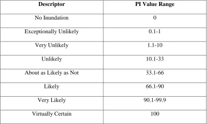
The cumulative probability of inundation (PI) can then be obtained by using the Z-score to calculate the corresponding probability from the cumulative (one tail) normal distribution (Schmid et al., 2014). The resultant spatially continuous inundation measure was categorised and mapped according to descriptors adapted from the
Table 2: Probability of Inundation Descriptors (after Mastrandrea et al., 2010)
Descriptor PI Value Range
No Inundation 0
Exceptionally Unlikely 0.1-1
Very Unlikely 1.1-10
Unlikely 10.1-33
About as Likely as Not 33.1-66
Likely 66.1-90
Very Likely 90.1-99.9
Virtually Certain 100
The Hydrologically Correct Bathtub Model & Monte Carlo Simulation
(HBM+MCS Method)
Monte Carlo Simulation (MCS) is a form of probabilistic analysis that has been used to model the effects of error in GIS (Fisher, 1991; Openshaw et al., 1991). MCS allows an assessment of uncertainty in inundation model outputs through the addition of
probability distributions to replace single values (Fisher, 1991), giving an indication of the effect of error in the input data (Openshaw et al., 1991). Similar iterative
approaches, based on MCS, have been applied to GIS error/uncertainty studies (Fisher, 1991; Lanter & Veregin, 1992; Holmes et al., 2000).
In such approaches, the original DEM is considered only one possible realisation of the true elevation. Further DEM realisations are produced by adding randomly
𝐿𝐸95𝑍 = 1.96 ∗ 𝑅𝑀𝑆𝐸𝑧 (3)
The use of the LE95 has become a commonly used representation of vertical error (Gesch, 2009, 2013), and has been applied to SLR uncertainty studies (Santillan & Makinano-Santillan, 2017) in the absence of the actual distribution of error being
known. Although the LE95z is property of the normal distribution, we are using it in this context simply to attempt to account for the fact that the RMSE is not a precise
quantification of error, and that the LE95z at least provides a more realistic range within which the actual (unknown) DEM error is likely to be located. The linear error at 95% confidence for the DEM in our study is 0.294m.
In the absence of any additional information relating to how vertical error might vary spatially in response to other factors, we assumed that error at each cell could vary up to the maximum in either direction, i.e., we have chosen to sample from the LE95z bounds uniformly This replicates The US Nature Conservancy Method (TNC) (Gilmer and Ferdana, 2012) except that where they use the RMSE, we have used LE95Z.
Our rationale for selecting a uniform distribution is that Schmid et al. (2014) present evidence that error may not be normally distributed in coastal environments. Sefercik et al. (2015) similarly show for their inland site that errors were normal for shorter vegetation, but were not for taller vegetation. Since the location and land cover of ground control points has not been provided and we have no other information about error, drawing from a uniform distribution, rather than a normal distribution, is more conservative. Five hundred individual randomised error fields with uniformly
distributed values between -0.294m and +0.294m were therefore created for both
Reuter et al., 2009; Leon et al., 2014), selecting this or any other averaging window would be an arbitrary decision, therefore no attempts were made to recreate the spatial structure of error. Each randomised error field was added to the original DEM creating a series of 500 new, equally valid, realisations of elevation.
The hydrologically correct bathtub model, widely used in SLR assessments (van de Sande et al., 2012; Sahin, 2014), was used to model inundation. The original bathtub model approach assumed that any areas with elevation values below the SLR projection should be classified as ‘flooded’ (Curtis & Schneider, 2011). An enhancement to this approach requires spatial continuity between the ocean and flooded areas for them to be classified. This approach is known as the hydrologically correct bathtub model and allows for a more representative model of surface flooding (Sahin, 2014). Each
elevation realisation, for both estuaries, was used as the input to a hydrologically correct bathtub model as presented below.
Firstly, the local HAT (SHAT) was added to the H++ scenario for Lyme Bay (SCC) (1.42m) to establish the inundation surface (S) (Equation 4):
𝑆 = 𝑆𝐻𝐴𝑇+ 𝑆𝐶𝐶 (4)
𝑆𝐹𝑙𝑜𝑜𝑑 = {𝐸 > 𝑆,0 𝐸 ≤ 𝑆,1∗ 𝐶𝑖 (5)
Where E is the elevation of a given cell, C represents connectivity (1 =
connected, 0 = not connected) and i is the connectivity rule (in this case the eight-side rule). The 500 SFlood surfaces were combined, and at the cell scale, the number of counts of SFlood = 1 represents the frequency of inundation, which we take to be a measure of the probability of inundation (PI) (Equation 6).
𝑃𝐼 = [∑𝑛𝑖=1𝑆𝐹𝑙𝑜𝑜𝑑
𝑛 ] ∗ 100 (6)
Where n is the number of DEM iterations, and PI is the probability of inundation expressed as a percentage. Areas which produced PI values of 0 represent those where no flooding occurred in any of the iterations, while a PI value of 100 represents areas which flooded in all iterations. Both areas represent certainty (either inundated or not inundated). Areas marked as flooded in some iterations, and not in others define a zone of inundation uncertainty. Low PI values represent low occurrence of inundation across the iterations and thus higher uncertainty in the flood extent and vice versa. Probability of inundation was mapped using the same class descriptors as mentioned earlier (Table 2).
Phase 2: Developing a Predictive Relationship between Elevation & Uncertainty
Unlike in watershed modelling, where multiple flow directions need to be considered, the flow of coastal inundation is primarily dependent on elevation (Poulter & Halpin, 2008). It stands to reason that in a situation of gradually increasing shoreline elevations, vertical error will give rise to some inundation uncertainty at the upper end of the shoreline elevations. It follows that if a site was selected that had a sufficiently
it should be possible to define a generalised relationship between elevation and
inundation, assuming a consistent local datum. Modelling inundation uncertainty using a MCS approach and a hydrologically correct bathtub model is computationally
intensive, and having a generalised relationship would provide a much quicker
indication of inundation uncertainty when applied to other areas. The advantage of full, iterative hydrologically correct bathtub modelling is that the protection effects of shoreline defences can be represented, which may be lost in the application of a generalized relationship. This poses questions about the trade-off between
computational effort against efficiency, and reasonable representation. This was the focus of the second phase of the research.
For each elevation in the original DEM (expressed relative to Ordnance Datum), the corresponding range in probability of inundation was plotted. Ordinarily one would expect high probability for low elevations, and lower probability (higher uncertainty) for higher elevations. However, for some lower elevations a low probability of
Results
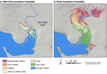
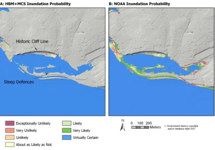
Phase 1: Modelled Inundation Uncertainty
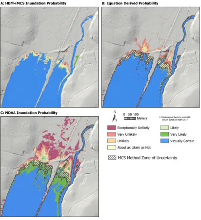
Figures 1 and 2 show the uncertainty surface arising from the respective modelling approaches in two contrasting topographies of the Exe Estuary (Figure 1 - flatter, Figure 2 - steeper). In all instances, the minimum extent of the waterbody of each estuary under climate change is clearly defined by the ‘virtually certain’ class. Depicted beyond this flood extent are zones of inundation uncertainty, which vary in extent depending on the method used. In the case of the hydrologically correct bathtub method (Figures 1A and 2A) the zone of uncertainty is smaller than that produced by the NOAA method
(Figures 1B and 2B) . However, it is evident in both locations that increases in
inundation uncertainty generally conform to increases in elevation. Local slope is also important, for example the zone of uncertainty is narrow where shoreline slopes are steep (Figure 2), but broadens where shoreline profiles are flatter, for example location B at the head of the estuary.
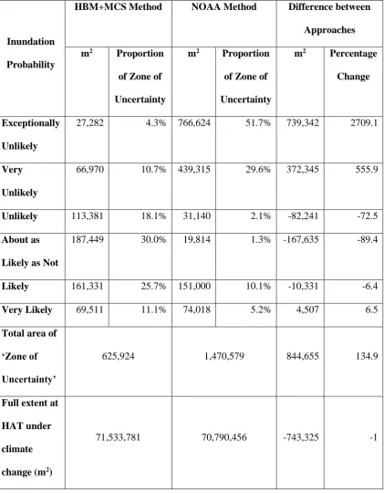
Table 3: Comparison of PI Likelihood Classification between the NOAA Method and the MCS Method for the whole study area (Otter and Exe Estuaries)
Inundation
Probability
HBM+MCS Method NOAA Method Difference between
Approaches
m2 Proportion
of Zone of
Uncertainty
m2 Proportion
of Zone of
Uncertainty
m2 Percentage
Change
Exceptionally
Unlikely
27,282 4.3% 766,624 51.7% 739,342 2709.1
Very
Unlikely
66,970 10.7% 439,315 29.6% 372,345 555.9
Unlikely 113,381 18.1% 31,140 2.1% -82,241 -72.5
About as
Likely as Not
187,449 30.0% 19,814 1.3% -167,635 -89.4
Likely 161,331 25.7% 151,000 10.1% -10,331 -6.4
Very Likely 69,511 11.1% 74,018 5.2% 4,507 6.5
Total area of
‘Zone of
Uncertainty’
625,924 1,470,579 844,655 134.9
Full extent at
HAT under
climate
change (m2)
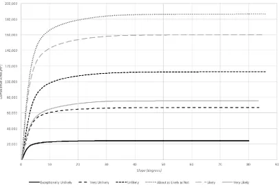
Figure 3 shows the relationship between local slope, inundation probability and associated inundated area. Each inundation class is comprised of almost a full range of slopes, but it is clear that most of the inundation is co-located with low slopes. This is especially the case for the class of greatest uncertainty (exceptionally unlikely), where approximately 75% of the total area of the class is co-located with slopes of 4.9 degrees or less.
Figure 3: Cumulative area occupied by different slopes at each inundation probability class for the whole study area.
Phase 2: Developing a Predictive Relationship between Elevation & Uncertainty
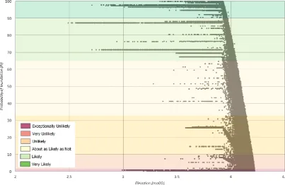
Figure 4 Elevation (maOD) versus probability of inundation (PI) for the Exe Estuary.
The general relationship between increasing elevation and decreasing
correct bathtub model; the distribution of uncertainty in this location reflects the distribution of potential elevations in relation to the height of the controlling structure.
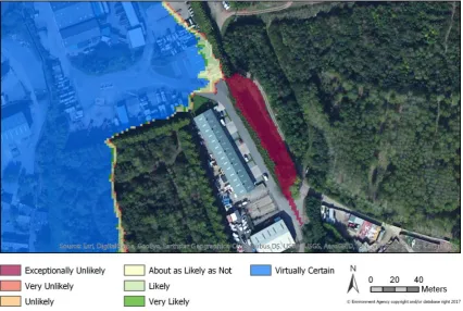
Figure 5: Impact of a protective structure, cell connectivity and DEM error in modelling probability of inundation.
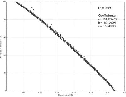
Figure 6 presents the maximum probability of inundation for any given elevation (the boundary curve of points on the right of Figure 4) which were extracted and
Figure 6: Maximum probability of inundation (PI) for each elevation (maOD) derived from the Exe Estuary.
𝑃𝐼𝑒𝑞𝑛 = 𝑎
(1+𝑒𝑏−𝑐𝑥) (Equation 7)
Where PIeqn is the generalised probability of inundation, x is the DEM-derived elevation and coefficients as defined in Figure 6.
Figure 7a shows the probability of inundation (PI) determined by the
upper centre of Figure 7b that is not shown as inundated in Figure 7a. This is an area of low topography behind a protective structure which does not appear in Figure 7a because although it is at low elevation, it is not hydrologically connected until the height of the protective structure is exceeded.
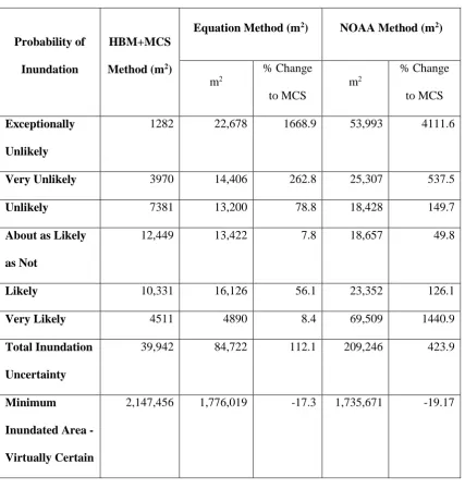
[image:22.595.92.505.188.641.2]Table 4 compares the area of inundation (m2) for each probability class and according to each of the three methods.
Table 4: Comparison of Uncertain Area in Modelled and Predicted Surfaces for the Otter Estuary
Probability of
Inundation
HBM+MCS
Method (m2)
Equation Method (m2) NOAA Method (m2)
m2 % Change to MCS m2 % Change to MCS Exceptionally Unlikely
1282 22,678 1668.9 53,993 4111.6
Very Unlikely 3970 14,406 262.8 25,307 537.5
Unlikely 7381 13,200 78.8 18,428 149.7
About as Likely
as Not
12,449 13,422 7.8 18,657 49.8
Likely 10,331 16,126 56.1 23,352 126.1
Very Likely 4511 4890 8.4 69,509 1440.9
Total Inundation
Uncertainty
39,942 84,722 112.1 209,246 423.9
Minimum
Inundated Area -
Virtually Certain
2,147,456 1,776,019 -17.3 1,735,671 -19.17
Discussion
We have used three approaches to represent coastal inundation which also incorporate representation of uncertainty arising from vertical error in the DEM. The most
required is an inundation surface, a DEM and the RMSE. From this a corresponding inundation uncertainty surface can be visualised according to user defined classes. When applied to the Exe and Otter Estuaries, this method delineates the widest extents of uncertainty. Unlike the HBM+MCS method, the NOAA method does not inherently accommodate the problem of mapping non-hydrologically connected areas, but avoids the computational time associated with the iterative HBM+MCS method (which includes connectivity assessment). In an attempt avoid the computationally intensive HBM+MCS method we test a regression approach which is straightforward to apply, but has limitations in that it identifies low elevation areas behind protective structures as areas of inundation uncertainty. Our regression approach identifies areas of inundation uncertainty intermediate between those of the NOAA and HBM+MCS methods, but is reliant on the HBM+MCS approach having been undertaken for a representative area with a similar HAT and SLR projection.
While superficially the choice between these approaches might rest on decisions about time and computational resources, we suggest that the differences between them are much more strongly related to their underpinning assumptions and associated value judgements. In particular, (i) how DEM error is measured and reported when published, (ii) the extent to which assumptions are made about the distribution of error, both at a point and across a surface, and (iii) how the resultant inundation probability surface is classified, and where one defines flood extent for practical purposes.
intended to be represented in the RMSE. In practice, this is calculated by selecting a number of ground control points (GCPs) and then comparing the DEM cell values at these locations to those surveyed (Wechsler, 2007). The errors encapsulated in the RMSEz and RMSExy scores thus represent deviation from the true measured values. This raises the question of the choice of GCPs, their coverage and suitability for all coastal areas.
In the US, The Federal Emergency Management Agency (FEMA) data quality assurance specifications (2003) require assessment of error across several classes [(a) open terrain, (b) urban or built-up infrastructure, (c) forest, (d) scrub-shrub, (d) weeds, tall grass and crops]. In practice, and even for coastal data, few ground control points are selected within coastal marsh environments, and it is assumed that category (d) would reasonably account for salt marsh (Schmid et al., 2011). Although one might intuitively anticipate higher errors for complex vegetation such as forests, Schmid et al. (2011) show that errors in salt marsh vegetation can be considerable. The structure of salt-marsh vegetation makes differentiation between ground and vegetation surface challenging, leading to vertical errors in the form of a positive bias (Schmid et al. 2011). Publishers of DEM products will usually provide a RMSE, and increasingly RMSEz and RMSExy. However further details such as the number, location and landcover in which the CGPs are located are usually not provided, as is the case with the composite DEM used for this analysis. A first question for any users of these datasets for coastal applications needs to be whether the stated RMSE adequately represents the specific errors associated with various coastal landcovers. It should be noted that some of these errors can be overcome by more judicious choices in LiDAR data observation
that for their study resulted in a reduction in bias of 12cm and an improvement in vertical accuracy of 8cm in saltmarsh vegetation.
The second major consideration is concerned with assumptions about the
distribution of errors. Spatial accuracy data standards (e.g. the US National Standard for Spatial Data Accuracy (NSSDA)) have traditionally assumed that the errors in spatial data are normally distributed (Zandbergen, 2008). This presumption has been extended to LiDAR-derived DEMs, where some have suggested that in open terrain (as opposed to forests and difficult to penetrate areas), the data ‘have normally distributed errors’ (NOAA 2012:7), although it is not clear from this source whether this is in reference to horizontal errors, vertical errors, or both. Zandberg’s evaluation of the assumption of normality in several spatial datasets found strong evidence for non-normal distributions (Zandberg, 2008), and further suggested that, as a single statistic, the RMSE
insufficiently characterises the nature of positional error in some geographic data sets. In the specific case of positional error in LiDAR-derived DEMs, he suggested that these could be ‘approximated with a normal distribution of the original (positive and negative) vertical errors after removal of a small number of outliers’ (Zandberg,
2008:126). Blak (2006) suggests that assumptions of normality would overstate vertical errors when they are not normal.
reason why this method generates the largest areas of inundation in Figures 1, 2 and 7. This is likely to be an overestimation of inundation, but consistent with a conservative approach.
The HBM+MCS method makes a different set of assumptions relating to the practical implementation of the RMSE. One option, as implemented by Gilmer and Ferdana (2012), would be to constrain the elevation at any cell to be between (elevation + the RMSEz) on the upper limit and (elevation - the RMSEz) on the lower limit. In other words the ‘DEM estimated’ elevation surface can only vary from the true elevation by + or – the RMSE. Given that there is inevitably always some uncertainty with the validity of RMSE as a measure, we feel that a slightly more conservative approach is warranted. We therefore adopted the Gesch (2009) LE95 approach, where errors at 95% confidence are estimated (Equation 3). We recognise that in calculating these errors we are assuming the errors are normally distributed and not biased (Schmid et al. 2014). However this assumption is only being made in the HBM+MCS method to constrain the errors realistically between the narrower range of just +/- RMSE (i.e. Gilmer and Ferdana, 2012), and the unconstrained NOAA method, which uses the full distribution and therefore over-estimates inundation in very low probability areas.
generated randomly and uniformly but constrained within the assumed bounds of +/-LE95. There is of course no independent, objective, or ‘true’ estimate of
[image:28.595.92.504.323.575.2]inundation probability by which we can evaluate these methods. Furthermore, the point of this paper is not to recommend specific choices of distribution, but to rather highlight the consequences of necessarily having to make these choices. Choice of method must therefore be made on the basis how appropriate we feel the necessary associated assumptions are. A further advantage of the HBM+MCS over the NOAA method is that it incorporates hydrologically correct inundation, but at computational cost.
Figure 8: Cumulative frequency plot for the Exe Estuary showing the effect of an assumption of a normal distribution of RMSE (grey line) versus a uniform
Given the resource-intensive nature of HBM+MCS method, we considered whether it might be possible to generalise the relationship between elevation and inundation probability. This could then be used in nearby areas with similar conditions of HAT and future SLR, potentially limiting the extent of coastline for which full HBM+MCS would need to be undertaken. The fundamental assumption here is that the maximum probability of inundation at each elevation defines the generalised
The reference to ‘reasonable’ above brings into focus the final of the three major observations we would like to make; namely around classification, representation and selection of inundation extents for practical use and decision making. Although we have applied the same classification and associated descriptors across all methods, this is nevertheless a value judgement. Figure 9 shows the Otter Estuary with inundation probability reclassified into a binary ‘certain’ and ‘uncertain’ classification. This form of binary classification has been used in previous SLR uncertainty studies (NOAA, 2010).
With the NOAA method it is recommended that each study ‘should chose the percentile ranks (e.g. 75%, 80% or 95%) that make sense to differentiate between areas that have high uncertainty and those that seem well represented by the mapped output’ (Schmid et al., 2014: 559). In effect, and particularly given the conservative ‘over-estimation’ arising from the assumption of normality, this equates to a reasonable value-judgement being made as to how much of the mapped uncertainty we should take seriously for practical purposes. In the HBM+MCS method we embed a value judgment by constraining possible error to the LE95. Value judgements, particularly in the
absence of more detailed information relating to the distribution of error in DEM products, are therefore necessary, regardless of what method is used. The important consideration therefore, is that all assumptions and value judgements are considered explicitly during the analytical process, and communicated clearly on resulting maps and other outputs.
Conclusion
This study set out to explore how the stated vertical error of a publically available LiDAR-derived DEM might impact on defining estuary extents at HAT under future climate change. Relatively few studies have addressed this need, which is becoming increasingly urgent as publically available DEMs become more widespread and better integrated into longer term coastal zone planning. For our study, stated RMSEz was low and although this does translate into a zone of inundation uncertainty, these are not large areas. For this location therefore, DEMs of this stated quality are appropriate to inform coastal decision-making. However, additional uncertainty analysis by the methods proposed provides a basis for relatively more informed decisions..
identification arises from compound errors linked to tidal gauges, methods of
interpolation, modelling assumptions and the confidence associated with climate change related sea level projections. Additionally, storm surges and the uncertainty associated with estimating these magnitudes, can significantly increase inundation levels. Coastal managers should therefore be mindful of all these sources of error. A broader
consideration of all sources of error as recommended by Schmid et al. (2014) would likely significantly increase the zone of inundation uncertainty, so research to examine the compound effects of these errors is important. We evaluated a method currently used to visualise inundation uncertainty nationally in the US (NOAA method, Schmid et al., 2014), against a method, based on hydrologically correct bathtub modelling and perturbation of the DEM constrained by the stated error in a Monte Carlo simulation. The two methods produced similar coverage in the ‘virtually certain’ classification (with a difference of -1%). However, the NOAA method produced a much larger zone of uncertainty compared to our HBM+MCS method (with an increase of 134.9%). We also expressed the outcome of this modelling as a regression equation and explored the utility of this as a quick approach to map inundation uncertainty in adjacent areas.
decision to represent inundation uncertainty is too, a value judgment. Considerations of DEM error and associated metadata in published DEMs, is still an area of concern. We reiterate the call by Wechsler a decade ago, and more recently Gesch, that DEM vendors should be urged to provide information on DEM error beyond just the RMSE (Wechsler, 2007; Gesch, 2013). This would include metadata regarding location of ground control points and associated land cover, estimates of consolidated vertical error (CVA) for each land cover and ideally, more advanced error assessment approaches (e.g. Sefercik et al. 2015).
References
Bales, J.D., Wagner, C.R., Tighe, K.C. & Terziotti, S. 2007. LIDAR derived flood inundation maps for real time flood mapping applications, Tar River Basin, North Carolina. US Geological Survey Scientific Investigations Report 2007, 5032(1), 42-44.
Beven, K., Cloke, H., Pappenberger, F., Lamb, R. & Hunter, N. 2015. Hyperresolution information and hyper-resolution ignorance in modelling the hydrology of the land surface. Science China: Earth Sciences, 58(1), 25-35.
Blak, T. 2006. DEM quality assessment. In: Maune, D.F. (ed.), Digital Elevation Model Technologies and Applications: The DEM Users Manual, 2nd edition. Bethesda, MD: American Society for Photogrammetry and Remote Sensing, 425–477. Boin, A.T. & Hunter, G.J. 2007. What communicates quality to the spatial data
consumer. 5th International Symposium on Spatial Data Quality, Enschede, The Netherlands, June 13-15.
Chang, B. 2014. Modelling spatial variations of sea level rise and corresponding inundation impacts: A case study for Florida, USA. Water Quality, 6(2), 39-51. Chu-Agor, M.L., Muñoz-Carpena, R., Kiker, G, Emanuelsson, A. & Linkov, I. 2011.
Exploring vulnerability of coastal habitats to sea level rise through global sensitivity and uncertainty analysis, Environmental Modelling & Software, 26(5), 593-604.
Cooper, H.M. & Chen, Q. 2013. Incorporating uncertainty of future sea level rise estimates into vulnerability assessment: a case study in Kahului, Maui. Climatic Change, 121(2), 635-647.
Couclelis, H. 2003. The certainty of uncertainty: GIS and the limits of geographic knowledge. Transactions in GIS, 2(7), 165-175.
Coveney, S. & Fotheringham, S. 2011. The impact of DEM data source on prediction of flooding and erosion risk due to sea level rise. International Journal of
Geographical Information Science, 25(7), 1191-1211.
Curtis, K.J. & Schneider, A. 2011. Understanding the demographic implications of climate change: estimates of localised population predictions under future sea level rise. Population & Environment, 33(1), 28-54.
Daly, C. 2006. Guidelines for assessing the suitability of spatial climate data sets. International Journal of Climatology, 26, 707-721.
Dottori, F., Di Baldassarre, G. & Todini, E. 2013. Detailed data is welcome, but with a pinch of salt: accuracy, precision and uncertainty in flood inundation modelling. Water Resources & Research, 49(2), 6079-6085.
Environment Agency (2016), Environment Agency LiDAR Data: Technical Note [online]. Available from:
http://www.geostore.com/environment-agency/docs/Environment_Agency_LIDAR_Open_Data_FAQ_v5.pdf [Accessed 11/12/2016]
FEMA (Federal Emergency Management Agency). 2003. Map Modernization,
Guidelines and Specifications for Flood Hazard Mapping Partners, Appendix A: Guidance for Aerial Mapping and Surveying. Washington DC: FEMA.
Fisher, P. 1991. First experiments in view shed uncertainty: the accuracy of the view shed area. Photogrammetric Engineering & Remote Sensing, 57(10), 1321-1327. Fisher, P. & Tate, N.J. 2006. Causes and consequences of error in digital elevation
models. Progress in Physical Geography, 30(4), 467-489.
Fowler, R.A., Samberg, A., Flood, M., & Greaves, T.J., 2007. Topographic and terrestrial Lidar. In: Maune, D.F. (ed.), Digital Elevation Model Technologies and Applications, The DEM Users Manual, 2nd edition. Bethesda, Maryland: American Society for Photogrammetry and Remote Sensing, pp. 199–252. French, J.R. & Burningham, H. 2013. Coasts and climate: Insights from
Gesch, D.B. 2007, The National Elevation Dataset, in Maune, D.F. (ed), Digital Elevation Model Technologies and Application: The DEM user’s Manual, 2nd edition. American Society for Photogrammetry and Remote Sensing, Maryland. Gesch, D.B. 2009. Analysis of LIDAR elevation data for improved identification and
delineation of lands vulnerable to sea level rise. Journal of Coastal Research, Special Issue 53, 49-58.
Gesch, D.B. 2013. Consideration of Vertical Uncertainty in Elevation Based Sea Level Rise Assessments: Mobile Bay, Alabama Case Study. Journal of Coastal Research, Special Issue 63, 197-210.
Gilmer, B.F. and Ferdana, Z., 2012. Developing a framework for assessing coastal vulnerability to sea level rise in Southern New England, USA. In: Zimmermann, M. (ed.), Local Sustainability. Dordrecth, The Netherlands: Springer, pp. 25–26. Goodchild, M.F. 2010. Twenty-years of progress: GIScience in 2010. Journal of Spatial
Information Science, Vol.1, 3-20.
Hennecke, W.G. 2004. GIS modelling of sea level induced shoreline changes – two examples from south-eastern Australia. Natural Hazards, 31(2), 253-276. Hodgson, M.E. & Bresnahan, P. 2004. Accuracy of airborne Lidar- derived elevation:
Empirical assessment and error budget, Photogrammetric Engineering & Remote Sensing, 70(3), 331–339.
Hodgson, M.E., Jensen, J., Raber, G., Tullis, J., Davis, B.A., Thompson, G. & Schuckman, K. 2005. An evaluation of LiDAR-derived elevation and terrain slope in leaf-off conditions. Photogrammetric Engineering & Remote Sensing, 71(7), 817-823.
Holmes, K., Chadwick, I. & Kyriakidis, P. 2000. Error in a USGS 30 metre digital elevation model and its impact on terrain modelling. Journal of Hydrology, 223(2000), 154-173.
Jongman, B., Ward, P.J. & Aerts, J.C.J.H. 2012. Global exposure to river and coastal flooding: long term trends and changes. Global Environmental Change: Human and Policy Dimensions, 22(4), 823-835.
Lanter, D. & Veregin, H. 1992. A research based paradigm for propagating error in layer based GIS. Photogrammetric Engineering & Remote Sensing, 58(6), 825-833.
Li, Z. 1998. On the measure of digital terrain model accuracy. Photogrammetric Record, 14, 873-877.
Li, X., Rowley, R.J., Kostelnick, J.C., Braaten, D., Meisel, J. & Hulbutta, K. 2009. GIS analysis of global impacts from sea level rise. Photogramming & Engineering Remote Sensing, 75(2), 807-818.
Maune, D.F., Maitra, J.B. & McKay, E.J. 2007. Accuracy Standards & Guidelines, in Maune, D (ed.), Digital Elevation Model Technologies & Applications: The DEM User’s Manual, 2nd edition. American Society for Photogrammetry & Remote Sensing: Maryland.
Mastrandrea, M.D., Field, C.B., Stocker, T.F., Edenhofer, O., Ebi, K.L., Frame, D.J., Held, H., Kriegler, E., Mach, K.J., Matschoss, P.R., Plattner, G.-K., Yohe, G.W. & Zwiers, F.W. 2010. Guidance Note for Lead Authors of the IPCC Fifth
Assessment Report on Consistent Treatment of Uncertainties, Intergovernmental Panel on Climate Change (IPCC).
NOAA. 2010. Technical Considerations for use of Geospatial Data in Sea Level Change Mapping & Assessment, NOAA: Maryland.
Openshaw, S., Charlton, M. & Carver, S. 1991. Error propagation: A Monte Carlo Simulation, in Masserr & Blackemore (eds.), Handling Geographic Information: Methodology & Potential Applications, Longman Scientific & Technical: London.
Oswald, M.R. & Treat, C. 2013. Identifying sea level rise vulnerability using GIS: Development of a transit inundation modelling method, International Journal of Geoinformatics, 9(1), 1-10.
Poulter, B. & Halpin, P.N. 2008. Raster modelling of coastal flooding from sea level rise, International Journal of Geographical Information Science. 22(2), 167-182. Rahmstorf, S. 2007. A semi-empirical approach to projecting future sea level rise.
Science, 315(3), 368-370.
Reuter, H.I., Hengl, T., Gessler, P. & Soille, P. 2009. Preparation of DEMs for geomorphometric analysis, in Tomislav, H. & Hannes, I.R. (eds),
Geomorphometry: Concepts, Software, Applications, Elsevier: Washington, 87-120.
Rubinstein, R. 1982. Simulation and the Monte Carlo method. Wiley: New York. Sahin, O. 2014. Coastal vulnerability to sea level rise: A spatial and temporal
Santillan, J.R. & Makinano-Santillan, M. (2017), Elevation-based sea-level rise vulnerability assessment of Mindanao, Philippines: Are freely-available 30-M DEMs good enough?, The International Archives of the Photogrammetry, Remote Sensing and Spatial Information Sciences, Volume XLII-2/W7, 2017, ISPRS Geospatial Week 2017, 18–22 September 2017, Wuhan, China.
Sayers, P., Horritt, M., Penning-Rowsell, E. & McKenzie, A. 2015. Climate Change Risk Assessment 2017: Projections of Future Flood Risk in the UK, Sayers & Partners LLP: Watlington.
Schmid, K., Hadley, B. & Waters, K. 2014. Mapping and portraying inundation uncertainty of bathtub-type models. Journal of Coastal Research, 30(3), 548-561.
Schmid, K., Hadley, B.C. & Wijekoon, N. 2011. Vertical accuracy and use of topographic LIDAR data in coastal marshes. Journal of Coastal Research, 27(6A), 116–132.
Sefercik, U.G., Glennie, C., Singhania, A. 2015. Area-based quality control of aurborne laser scanning 3D models for different land classes using terrestrial laser
scanning: Sample survey in Houstan, USA, International Journal of Remote Sensing, 36(23), 5916-5934.
Shearer, J.W. 1990. The accuracy of digital terrain models, in Petrie, G. & Kennie, T.J.M (eds), Terrain modelling in surveying and civil engineering, Whittles Publishing: Caithness, 315-336.
Tucci, M. & Giordano, A. 2011. Positional accuracy, positional uncertainty, and feature change detection in historical maps: results of an experiment. Computers, Environment and Urban Systems, 35(6), 452-463.
van de Sande, B., Lansen, J. & Hoyng, C. 2012. Sensitivity of coastal flood risk assessments to digital elevation models. Water, 4, 568-579.
Wallentin, G. & Car, A. 2013. A framework for uncertainty assessment in simulation models. International Journal of Geographical Information Science, 27(2), 408-422.
Wechsler, S.P. 2007, Uncertainties associated with digital elevation models for
White, S.A., Parrish, C.E., Calder, B.R., Pe’eri, S. & Yuri, R. 2011. LIDAR-Derived National Shoreline: Empirical and Stochastic Uncertainty Analyses. Journal of Coastal Research, Special Issue 62, 62-74.
Zandbergen, P.A. 2008. Positional accuracy of spatial data: Non-normal distributions and a critique of the national standard for spatial data accuracy. Transactions in GIS, 12(1), 103-130.