Elsevier Editorial System(tm) for Computer Vision and Image Understanding
Manuscript Draft
Manuscript Number: CVIU-17-1R1
Title: Polarisation Photometric Stereo Article Type: Research paper
Keywords: Polarisation; photometric stereo; 3D reconstruction Corresponding Author: Dr. Gary Atkinson, PhD
Corresponding Author's Institution: University of the West of England First Author: Gary Atkinson, PhD
Order of Authors: Gary Atkinson, PhD
Abstract: This paper concerns a novel approach to fuse two-source
photometric stereo (PS) data with polarisation information for complete surface normal recovery for smooth or slightly rough surfaces. PS is a well-established method but is limited in application by its need for three or more well-spaced and known illumination sources and Lambertian reflectance. Polarisation methods are less studied but have shown promise for smooth surfaces under highly controlled capture conditions. However, such methods suffer from inherent ambiguities and the depolarising
effects of surface roughness. The method presented in this paper goes some way to overcome these limitations by fusing the most reliable
information from PS and polarisation. PS is used with only two sources to deduce a constrained mapping of the surface normal at each point onto a 2D plane. Phase information from polarisation is used to deduce a mapping onto a different plane. The paper then shows how the full surface normal can be obtained from the two mappings. The method is tested on a range of real-world images to demonstrate the advantages over standalone
Dear reviewers and editor,
I am very grateful for the time and consideration that you have devoted to reviewing my paper. I was delighted to hear that the comments were mostly positive but also greatly appreciate the constructive feedback. I have addressed the issues raised and feel this has improved the paper significantly.
Please find my response to specific comments attached separately. I shall look forward to hearing your decision.
Best regards, Gary Atkinson
Reviewer #1:
“1. Do you evaluate the influence of individual steps in the proposed framework, e.g., the azimuth estimation? Which module is the major part regarding the overall accuracy?”
This is a very interesting question! I have conducted some experiments where either the polarisation data (phase and degree of polarisation) or photometric stereo data (intensity) were simulated. This showed clearly that, for simple surfaces at least, it is photometric stereo that is the main limitation. This additional analysis is now described near the end of Section 4.1 in lines 425 to 435.
“2. How is the accuracy compared to utilizing conventional polarization methods such as [11][12]?”
I have compared some of the methods in the literature review more directly to the new method now (scattered throughout lines 61 – 78). As is often the case, direct and perfectly fair comparisons are difficult due to unspecified details in certain papers and different hardware requirements (e.g. multi-view vs. multi-source). The most similar method however, is now compared numerically on line 74. Less-quantitative pros and cons compared to the state-of-the-art are provided throughout the literature review.
“3. The hyperlinks of the figures & references did not work in current pdf?”
Apologies for this. I believe it is a result of the LaTeX compiler in the submission system, which I do not have access to. The links are working when pdfLatex is used offline. I will make absolutely certain the links are all working in the published version.
Reviewer #2:
“1. More evaluating in terms of normal accuracy
As the author also correctly claimed, that normal estimation accuracy cannot be completely reflected from the integrated surface. So, it makes more sense to show the normal comparison for Fig. 6 and Fig. 9. The author uses l2 error for several evaluations, but I think the angular error statistics makes the result more intuitively understandable in Figs. 4, 7 and 8.”
I agree that a little more consideration about the error metric used for each figure was necessary and have made some amendments accordingly:
- Fig 6 (now called Fig 7): I have left this particular figure as a depth graph because surface normal error (which both the reviewer and I agree is generally more representative) is evaluated in great detail afterwards. I feel it is useful to see overall depth errors at some point early in the results section. However, I can change this to normal angular error if the reviewer insists but I think that would not add much to the paper.
- Fig. 7 and 8 (now called 8 and 9): Converted to angular error as requested – good suggestion. Fig. 9 (now 10): Converted to normal error as requested. I have also formatted this graph in the same way as Fig. 10 (now 12) for ease of comparison. However, I have also included the depth error graph as a new figure (Fig 11 in the new version) to demonstrate the effects of large angular errors on depth estimation.
- I’m a little confused about the reviewer’s reference to Fig. 4 (now 5) as this is not a graph at all. However, I am confident that the changes above satisfy this comment.
“2. Specular reflection vs. specular interreflection
When analyzing Figs. 2 and 3, the author said in line 159 that the pi/2 flip is due to specular reflection. Specular reflection can indeed cause such a flip, but the scenario in Fig. 3 is mainly due to specular interreflection. Line 251 says both direct and inter-reflective specular reflection can cause such an effect. I suggest checking the consistency of this term, and make it clear throughout the paper. If possible, the author may also show an example due to specular reflection (e.g., by painting half of the diffuse sphere
I agree with the reviewer that there is some inconsistency in terminology between “specularity”, “inter-reflection”, etc. I have therefore tidied up the terminology throughout the paper and used the terms “direct specularity” or “specular inter-reflection” throughout or simply used the term
“specular/specularity” where the text refers to either type. In addition, I have added a figure (Fig. 4 in the new version) to demonstrate a large direct specular reflection. This is explained in the last paragraph of Section 2.
“3. Minor issues
- Missing references:
[T. Ngo et al., Shape and Light Directions from Shading and Polarization, CVPR 15]: this paper combines photometric stereo and shape from polarization.
[W. Smith et al., Linear Depth Estimation from an Uncalibrated, Monocular Polarisation Image, ECCV 16]: this is one of the latest paper proposing a purely polarization based approach for complete normal estimation.”
Thank you for suggesting these references. I strongly agree that these deserve a mention and have covered both in Section 1.1 (between lines 72 and 85).
“- It should be highlighted in the conclusion that a major limitation of using two-source photometric stereo is that it cannot deal with non-Lambertian materials (it could be quite sensitive to material reflectance variation due to too few light sources). But shape from polarization is not that sensitive to reflectance properties and thus can deal with much more broader range of material types. I think combining with two-source photometric stereo somehow sacrifices such an advantage of shape from polarization.”
A method for surface normal recovery using photometric stereo and polarisation
Two source photometric stereo used for 2D normal estimation
Polarisation information used for azimuthal angle estimation
Unknowns in normals due to ambiguities are resolved via region growing across surface
Method is proven robust to specular inter-reflections and evaluated extensively
Polarisation Photometric Stereo
Gary A. Atkinson
Bristol Robotics Labratory
Department of Engineering Design and Mathematics University of the West of England, Bristol
BS16 1QY UK
Abstract
This paper concerns a novel approach to fuse two-source photometric stereo
(PS) data with polarisation information for complete surface normal recovery
for smooth or slightly rough surfaces. PS is a well-established method but is
limited in application by its need for three or more well-spaced and known
illumination sources and Lambertian reflectance. Polarisation methods are less
studied but have shown promise for smooth surfaces under highly controlled
capture conditions. However, such methods suffer from inherent ambiguities
and the depolarising effects of surface roughness. The method presented in this
paper goes some way to overcome these limitations by fusing the most reliable
information from PS and polarisation. PS is used with only two sources to
deduce a constrained mapping of the surface normal at each point onto a 2D
plane. Phase information from polarisation is used to deduce a mapping onto
a different plane. The paper then shows how the full surface normal can be
obtained from the two mappings. The method is tested on a range of real-world
images to demonstrate the advantages over standalone applications of PS or
polarisation methods.
Keywords: Polarisation, photometric stereo, 3D reconstruction
1. Introduction
Three-dimensional surface reconstruction/analysis has been a major goal of
computer vision for many years. There have a plethora of methods proposed
in the last few decades, each with their unique pros and cons. For example,
binocular stereo [1] applies at any range and is inexpensive but inappropriate for
5
featureless surfaces. By contrast, time-of-flight cameras [2] are known to operate
on a variety of scenes at high speed but suffer at long range. This paper uses
a fusion of photometric stereo (PS) and polarisation vision aimed at featureless
surfaces at close range: a goal that typically requires expensive methods that
use lasers or active illumination, else only operate at low resolution.
10
The proposed method initially applies a form of two-source PS to estimate
part of the surface normal. This is much more applicable to real world
appli-cations than most PS methods that require three or more sources on different
illumination planes. Polarisation information is then used in conjunction with
the PS-based estimates in order to fully constrain the normals at each pixel.
15
The paper therefore represents a significant step forward towards commercial
robotics applications able to exploit a largely untapped area of light: that of its
polarisation state.
This paper starts by reviewing the state-of-the-art in three-dimensional
sur-face estimation using polarisation. Then, in Section 2, the key background
20
theory from Fresnel Theory and polarisation imaging is provided. The novel
re-construction algorithm is described in detail in Section 3. Experimental results
and conclusions are provided in Sections 4 and 5 respectively.
1.1. Related work
One of the early proposed methods for surface shape estimation was that
25
of shape-from-shading, which aims to acquire geometry from an image using
intensity information only [3]. Due to its single-view and passive nature, it is
an attractive goal and does not suffer from the limitations of the above
ex-amples (binocular stereo and time of flight). Unfortunately, the method is
known to be ill-posed due to the bas-relief ambiguity and other reasons [4]. PS
30
was proposed as a means to overcome the ambiguities at the expense of the
need for three or more light sources, of known direction, illuminated separately
method become useful in many applications due to the relative ease of high
speed camera–illumination synchronisation [5]. However, the applications are
35
still highly limited due to the need for at least three sources. For example, for
many land-based robotics applications, it is easy to include two light sources
(to the far-left and far-right of the robot), but it is difficult to position a source
high above the ground. That said, Zhang et al. [6] apply geometric assumptions
to force a solution for smooth surfaces with two-source PS.
40
A less-studied approach to 3D vision problems is that ofpolarisation vision.
That is, the use of the polarisation state of reflected light to deduce surface
information [7]. As with the field of hyperspectral imaging, the method taps into
an entire set of information about the incoming light (polarisation state/spectral
composition) that a standard greyscale or RGB camera is unable to. Thus, one
45
may argue that a great deal of potentially useful information about the incoming
light is lost in standard vision techniques. Of course, the additional information
available from polarisation and hyperspectral imaging systems comes at the cost
of more expensive and often slower capture hardware.
Most previous computer vision research using polarisation uses Fresnel
the-50
ory applied to specular reflection [8]. The theory tells us that initially
unpo-larised illumination undergoes a partial linear polarisation process upon
reflec-tion from surfaces. The specific properties of the polarisareflec-tion correlate to the
relationship between the surface orientation and the viewing direction [7, 9].
Unfortunately, there are inherent ambiguities present (see Section 2) and the
55
refractive index of the target is typically required. Further, different equations
are required to model reflection if adiffuse component is present.
Miyazaki et al. [10], Atkinson and Hancock [11] and Berger et al. [12] all use
multiple viewpoints to overcome the ambiguity issue. In [10], specular reflection
is used on transparent objects – a class of material that causes difficulty for most
60
computer vision methods. In [11], a patch matching approach is used for
dif-fuse surfaces to find stereo correspondence and, hence, 3D data. Results are of
comparable quality to this paper, but cannot easily handle
is applied. Taamazyan et al. [13] use a combination of multiple views and a
65
physics-based reflection model to simultaneously separate specular and diffuse
reflection and estimate shape (Miyazaki et al. [14] also separate reflection
com-ponents but only as a pre-processing step).
Drbohlav and ˇS´ara [15, 16] use PS (as in this paper) but with linearly
po-larized incident illumination. Atkinson and Hancock [17] also use PS but with
70
more light sources and less resilience to inter-reflections than the method of this
paper. Ngo et al. [18] propose a similar combined polarisation/two-source PS
method to the one presented in this paper with optimal results reported to be
of the order 2◦ error from ground truth (this paper manages of 3−4◦).
How-ever, the Ngo paper focuses on estimating the lighting directions rather than
75
addressing complications due to specularities/inter-reflections (which was a key
motivation here).
Garcia et al. [19] use a circularly polarised light source to overcome the
ambiguities while Morel et al. [20] extend the methods of polarisation to metallic
surfaces by allowing for a complex index of refraction. Smith et al. [21] assume
80
a known constant refractive index and albedo but are able to pose the problem
as a system of linear equations. This allows to directly deduce depth up to a
concave/convex ambiguity in the presence of both diffuse and specular reflection.
Furthermore, the method is successfully applied to conditions of uncontrolled
illumination and only relies on a single view.
85
In an effort to overcome the need for the refractive index, Miyazaki et al.
con-strain the histogram of surface normals [14] while Rahmann and Canterakis
[22, 23] use multiple views and the orientation of the plane of polarisation for
correspondence. Huynh et al. [24] actually estimate the refractive index using
spectral information. Kadambi et al. [25] propose a method to allow polarisation
90
information to be combined with alternative depth capture methods resulting
1.2. Contribution
The motivation for this paper relates to the following weaknesses of existing
methods in related areas: firstly the need for three light sources in PS; secondly
95
the multiple ambiguities in polarisation; and thirdly the complexities due to
specular inter-reflections and diffuse reflection in both PS and polarisation. The
contributions are as follows:
• Exploit the advantages of PS methods but using only two sources.
• Reduce the dependency of PS on light source knowledge.
100
• Use a combination of PS and polarisation data with a novel region
grow-ing algorithm to deduce the full 3D surface normals of an object in the
presence of specular inter-reflections (assuming that the majority of the
surface is not specularly reflecting). The method is also somewhat robust
to direct specularities, depending on their relative intensity compared to
105
the diffuse component.
• Avoid the need to know or estimate the refractive index.
As stated earlier, it is thought that overcoming these limitations allows a
signif-icant step towards the usage of polarisation information in real-world robotics
applications.
110
2. Polarisation Vision
This paper is based on the premise that light undergoes a partial
polarisa-tion process upon reflecpolarisa-tion from smooth surfaces. Consider the experimental
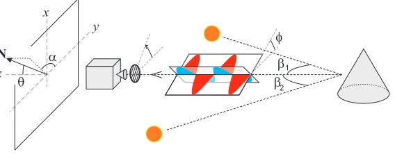
arrangement shown in Fig. 1, which is used for all of this work. Fresnel
re-flectance theory [8] is able to quantify the polarisation process that occurs when
115
initially unpolarised incident light is reflected towards the camera. The reflected
light can be parametrised by three values. First is the intensity,I, of the light.
Second is the phase angle,φ, which defines the principle angle of the electric field
component of the light as shown in the figure. Finally, the degree of
polarisa-tion,ρ, indicates the level of polarisation from 0 (unpolarised) to 1 (completely
120
x
z
y
b2 f
b q
a
N
1
Figure 1: Arrangement and definitions. Two polarisation images are acquired using the camera and rotating polariser. Each image has a different source illuminated. The surface normal,N, is defined by its zenith angle,θ, and azimuth angle,α.
As explained elsewhere in the literature [7, 26], for specularly reflected light
the phase angle aligns perpendicularly to the projection of the surface normal
onto the image plane. Assuming that the Wolff subsurface scattering model [27]
applies, diffuse reflection causes parallel alignment. Since there is no
distinc-125
tion in phase angle shifts ofπ radians, there are therefore four possible surface
azimuthal angles (defined in Fig. 1) for an unknown reflectance type:
α∈
φ, φ+π
2, φ+π, φ+ 3π
4
where 0≤φ < π (1)
The degree of polarisation contains information principally related to the
zenith angle of the surface. Unfortunately, the relationship between zenith
an-gle and degree of polarisation varies substantially between specular and diffuse
130
reflection and depends on the refractive index of the reflecting surface, which is
typically unknown [26]. For this reason, its use for surface normal estimation is
avoided in this paper. The method does however use the degree of polarisation
as a measure of reliability of the phase data: any phase data with a
correspond-ing degree of polarisation below a threshold (fixed at 1%) is deemed unreliable
135
due their correspondingly high associated noise levels.
The method described in the next section requires two polarisation images of
an object for input (a single polarisation image comprises a separate intensity,
phase and degree of polarisation value for each pixel). There are now several
commercially available cameras that capture such data directly such as the
[image:11.612.167.451.126.237.2]Fraunhofer “POLKA” [28]. The POLKA has a sensor divided into 2×2 cells,
with each element sensitive to light of a given electric field orientation (0, 45◦,
90◦ and 135◦). If the intensities measured for these angles are called I0, I45,
I90 andI135 respectively, then the polarisation data for each cell is calculated
via the Stoke’s parametersS0, S1 andS2 (assuming no circular polarisation is
145
present) [8]:
Stoke’s parameters:
S0=
I0+I45+I90+I135
2 (2)
S1=I0−I90 (3)
S2=I45−I135 (4)
Polarisation image data:
150
I=S0 (5)
φ= 1
2arctan2
S2 S1
(6)
ρ=
p
S2 1+S22 S0
(7)
where arctan2 is the four quadrant inverse tangent [29].
Raw data for this paper were captured using a Dalsa Genie HM1400 camera
with a motor-controlled circularly polarising filter in front of the lens. The motor
155
rotated the filter to angles of 0, 45◦, 90◦ and 135◦between each image capture,
after which (2–7) were applied to calculate the polarisation image; following a
similar method to the POLKA. A circular filter was used, rather than linear, in
order to minimise effects of any inter-reflections in the lens (Schneider KMP-IR
Xenoplan 23/1,4-M30,5) [30]. The rotating polariser method is clearly much
160
slower (but cheaper) than using the POLKA (or similar products) and thus
restricts application to stationary objects. However, the rest of the paper is
independent of the capture method and so could easily be applied to moving
objects if such cameras were used with this method in the future.
Examples of the three components of the polarisation image for a white
165
snooker ball are shown in Figs. 2 to 4. Note that the intensity is normalised
ball illuminated by a single small white LED placed close to the camera and
blackout curtains surrounding the ball to diminish all inter-reflections from the
environment. The reflection is therefore of diffuse type throughout the surface
170
and so the first or third solutions to (1) must be true for all pixels.
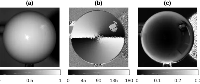
For Fig. 3, a plain matte white board was placed behind the ball. A sudden
phase shift is present near the occluding contours of the ball due to an
inter-reflection from the board. Since this region is effectively undergoing a specular
inter-reflection, the second or fourth solutions to (1) are true. By contrast,
175
the first or third solutions are true for the rest of the ball, which is exhibiting
diffuse reflection. Note also, that the degree of polarisation is higher near the
inter-reflection on the right-hand side of the ball. This is also predicted by the
reflection theory but is of less significance to this paper [26]. The noise-ridden
background to Fig. 3 is due to the very low degree of polarisation for the board
180
and the shadow cast by the ball; neither of which are of significance here.
The polarisation image in Fig. 4 includes an extended light source located to
the upper-right of the ball. The phase shift is clearly present here, demonstrating
the specular nature of the direct reflection. Careful examination of the degree of
polarisation demonstrates some inter-reflections from the laboratory are present
185
just below the main specularity. Since the intensity from these inter-reflections
is very low, the dominant reflection type is diffuse there.
3. Method
The approach can be broadly divided into the following steps assuming that
the starting point is two full polarisation images corresponding to the two light
190
source locations shown in Fig. 1.
1. Extract estimates of 2D (y-z) surface normals from two-source PS.
2. (a) Extract estimates of 2D (x-y) surface normals from polarisation aided
by PS.
(b) Disambiguate spurious data or specular inter-reflections (or,
poten-195
(a)
0 0.5 1
(b)
0 45 90 135 180
(c)
[image:14.612.139.473.157.300.2]0 0.1 0.2 0.3
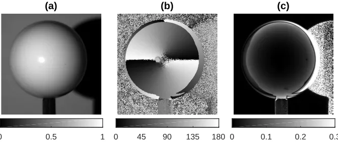
Figure 2: Example polarisation image of a white snooker ball with no inter-reflections and only one specularity (which is saturated in the image). (a) IntensityI, (b) phase angleφ, (c) Degree of polarisation,ρ.
(a)
0 0.5 1
(b)
0 45 90 135 180
(c)
0 0.1 0.2 0.3
[image:14.612.140.472.422.562.2](a)
0 0.5 1
(b)
0 45 90 135 180
(c)
[image:15.612.141.472.126.265.2]0 0.1 0.2 0.3
Figure 4: Example polarisation image of a white snooker ball with a direct specularity from an extended source and a sequence of uncontrolled environmental inter-reflections on the right-hand side. (a) IntensityI, (b) phase angleφ, (c) Degree of polarisationρ.
3. Combine data from each modality to obtain 3D (x-y-z) surface normals.
The first step essentially applies a 2D version of PS to obtain a 2D surface
normal at each pixel. This is not merely a projection of the 3D normal onto
they-z plane but rather a vector representing one particular degree of freedom
200
of the orientation of the surface at each point. The second step uses the
po-larisation phase angle of the incoming light and assumes diffuse reflection (for
now) to estimate a 2D version of the surface normal in thex-y plane. PS data
is applied to disambiguate most of these vectors but region growing is needed
where specularities occur or where previous disambiguation is deemed incorrect
205
(as defined in Section 3.2.2). Finally, the information above is combined to form
a 3D surface normal map.
3.1. Application of PS
The aim here is to use the method of PS to estimate a 2D normal in they-z
plane at each point. To do this, the original methodology of Woodham [31] is
210
adapted to two images in order to obtain a set ofnnormals as follows:
N(ps)i =
Ny,i(ps)
Nz,i(ps)
n i=1 ←
−cos(βR) cos(βL)
sin(βR) −sin(βL) IL,i IR,i
where the angles βL and βR are defined in Fig. 1 and the suffix “ps” is a
reminder that these estimates are from photometric stereo. The “←” symbol
is used throughout this paper to refer to variable assignment. The vectors are
then normalised into unit vectors in preparation for fusion with the polarisation
215
data.
One of the aims of this paper is to ensure that the method is robust to
disruptions in illumination. For example, standard PS yields poor results if one
source appears much brighter than the other or if the distance to the target
object varies (as this affects the light source vector). The results for this paper
220
were obtained with accurately positioned illumination so this potential issue
does not manifest. However, it is possible to use the phase information from
polarisation to calibrate the light source intensities assuming a linear (or at
least known) camera response profile. This is done by scaling the intensities
such that areas where φ = 90◦ or 270◦ have equal I values. Further, it is
225
worth noting at this point that the distance-to-target issue is less pronounced
here than standard PS since only thez-component of the normal is affected by
incorrect source vectors.
3.2. Application of polarisation vision
This section describes the method to estimate 2D normals in thex-yplane. It
230
assumes that the method for polarisation image acquisition described in Section
2 has been applied to arrive at corresponding intensity, phase and degree of
polarisation values for all npixels: {Ii, φi, ρi}ni=1. This section also makes use
ofnN(ps)i on
i=1
. This part of the algorithm is in two parts, the code for which is
summarised in Algorithm 1.
235
The raw data yields two estimates of polarisation values for each pixel (one
corresponding to each light source direction). In theory, the data should be
identical between each polarisation image, except for the locations of
speculari-ties and shadows. The proposed algorithm first forms a new polarisation image
corresponding to what is deemed the most reliable data for each pixel. Two
240
corresponding to the highest intensity at each point, (2) use the polarisation
data from the image corresponding to smallest deviation between raw data and
the transmitted radiance sinusoid [26]. While the latter approach is perhaps
more technically sound, it was experimentally determined that the final quality
245
of results were very similar between the two approaches. For this reason, the
former more computationally efficient approach was used for the remainder of
the research.
3.2.1. Initial azimuth estimation
This is covered by the first three lines of Algorithm 1. The first line applies a
250
sharpening operator to the phase data. The reason for this that the subsequent
specularity detection/disambiguation algorithm (“localAlign”) is more reliable
in the presence of sharp transitions between specularities and diffuse regions.
An alternative to this is to increase the definition of a neighbourhood in the
subsequent function, allowing the method to bridge over any gradual transitions.
255
The method makes the initial assumption that all surface normal projections
Algorithm 1Input: nφi, ρi,N (ps) i
on
i=1 Output:
n N(po)i o
n
i=1
1: {φi} ←sharpen ({φi})
2: {αi} ←
φi ∀i|
Ny,i(ps)<0∧φi>π2
∨Ny,i(ps)>0∧φi< π2
φi+π otherwise
3:
N(po)i =
Nx,i(po)
Ny,i(po)
n i=1 ←
−sinαi
cosαi
∀i
4: {Ri} n i=1←
1 ∀i|isBorderPixel(i)∨ρi<0.01
0 otherwise
5: while[More seed points?] do
6: j←Get seed point
onto thex-y (image) plane are aligned parallel to, or anti-parallel to, the phase
angle, as predicted by the theory for diffuse reflection covered in Section 2. Line
2 sets the azimuthal angle, α, of each point accordingly. Whether said
projec-tions are parallel or anti-parallel depend on the best match to the estimated 2D
260
normal from PS. Line 3 simply generates a set of 2D surface normals on the
x-y plane using the calculated azimuth angles. The suffix “po” reminds us that
these estimates are primarily from polarisation.
3.2.2. Final azimuth estimation
This is covered by the last four lines of Algorithm 1. It is expected that
265
most of the normals will be correct at this point. However, it is likely that some
regions of the image will be incorrect due to one of the following reasons:
• Diffusely reflecting regions with incorrect disambiguation. This is typically
whereNy(ps)≈0, meaning the initial disambiguation is not robust. These
regions have an azimuth error orπradians.
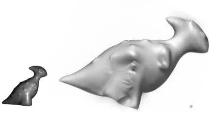
270
• Specular (direct or inter-reflective) regions. In these areas the azimuth
angle error isπ/2 radians, as predicted by the theory described in Section
2.
Lines 4 to 7 of Algorithm 1 are intended to address these possibilities, while
enforcing (1). First, a set of pixels,{Ri} n
i=1 are determined that shouldnot be
275
further considered by the algorithm. In the first instance, these pixels
corre-spond to:
• Image border pixels: purely to avoid slowing down the algorithm with
numerous conditional statements.
• Those with very low (<1%) degree of polarisation: since these areas are
280
deemed to have too much noise to be of use.
Next, a seed point is chosen. This can easily be done either manually or
randomly using a point of high confidence (i.e where the degree of polarisation
is high and eitherNy(ps)0 orN
(ps)
Algorithm 2 “localAlign”.
Input: nN(po)i , Ri on
i=1
, j Output: nN(po)i
on
i=1
1: if [Rj = 1]then
2: return
N(po), R
3: Rj ←1
4: for[k←neighboursOf (j)]do
5: ∆α←arccosN(po)j ·N(po)k
6: if [small (∆α)]then
7: N(po) ←localAlign N(po), R , k
8: if [small (π−∆α)]then
9: N(po)k ← −N(po)k
10: N(po) ←localAlign
N(po), R , k
11: if
small π2 −∆α
then
12: Nrot←
0 1
−1 0
·N (po) k
13: if harccosN(po)j ·Nrot
<π 2 i
then
14: N(po)k ←Nrot
15: else
16: N(po)k ← −Nrot
17: N(po) ←localAlign
N(po), R , k
this point must be of diffuse reflection so may benefit from some heuristics-based
285
selection in future work. Assume for now that only one seed point is needed,
but note that the code permits more if necessary (e.g. for complicated shapes).
The rest of the process involves a recursive call to a region growing function,
The region growing works as follows (see Algorithm 2). First, the function
290
checks whether the point in question j should be considered by reference to
{Ri} (lines 1 and 2). On occasions whereRj = 1, the function call terminates.
Where this is not the case, pointj is added to{Ri}, i.e. so it is not considered
again (line 3). The remainder of the function is completed for each neighbour
of the point (line 4). The neighbourhood can be defined in multiple ways but a
295
simple 4-connected region is used for this paper.
Next, the angle between neighbouringx-ysurface normals is calculated, ∆α
(line 5). There are four possibilities for ∆α:
• ∆αis close to zero: assume both azimuth angles are correct, move fromj
to neighbouring point,k, and continue the process (lines 6 and 7).
300
• ∆αis close toπ: as above but assume azimuth disambiguation was
incor-rect so rotate byπ(lines 8 to 10).
• ∆α is close to π/2: rotate azimuth by π/2 since this region is likely
fol-lowing specular reflection. The direction of rotation is chosen to minimise
the angle between the normals atj and k. Again, move from j to kand
305
continue the process thereafter (lines 11 to 17).
• Otherwise: there could be a boundary of orientation so there is no reason
to believe a the azimuth estimate is erroneous.
The definition of “close” for this recursive function remains open for now but
only minor effects on results were observed as the threshold for closeness was
310
varied between 5◦ and 10◦.
3.3. Fusion of data into full 3D surface normals
The methods from the previous two sections give two sets of 2D surface
normals:
N(ps) on the y-z plane and
N(po) on the x-y plane. These can
be combined into a single 3D vector. First assume that the 2D vectors are
315
normalised such that the following is true for each point:
where the subscriptsiare omitted for the sake of brevity.
Denote the 3D surface normal at a particular point N = [Nx, Ny, Nz]T.
Further, choose the components estimated by polarisation forxand y so there
is only one unknown,Nz:
320
N= [Nx, Ny, Nz] T
=hNx(po), Ny(po), Nz iT
(10)
Normalising this vector to unit length gives:
n=
h
Nx(po), N (po) y , Nz
iT
p
1 +N2
z
=hn(po)x , n(po)y , nz iT
(11)
This can then be re-normalised such thatn(po)y 2
+n2z= 1, matching the form of
the 2D estimate from PS as in (9). For thez component specifically:
nz q
n(po)y 2
+n2 z
=Nz(ps) (12)
Substituting the components ofnfrom (11) and simplifying:
Nz(ps)= q Nz
Ny(po) 2
+N2
z
(13)
Rearranging:
325
Nz= N (po) y 1
Nz(ps) 2−1
!−1/2
(14)
where the|·| sign is used sinceNz must be positive. This means that the only
unknown in (10) is resolved and so the surface normal is fully determined.
As stated earlier, the regions of the images where the degree of
polarisa-tion is less that 1% are not used in the algorithm to ensure robustness. For
the results in the next section, bi-cubic interpolation was used to estimate the
330
normals for these areas. It was also found that improvements could be made
by interpolating over regions of very lowNy, although this was kept to a
min-imum. It is acknowledged however, that more sophisticated methods from the
The normals can be converted to depth using any of a number of integration
335
methods [32]. Since it is not the aim of this paper to develop a new
integra-tor, the well-established Frankot-Chellappa method [33] is primarily used for
this step. The method is fast and highly robust to noise, but can suffer from
over-smoothing. An alternative method that does not over-smooth is briefly
considered in Section 4.3.
340
4. Results
This section contains a detailed analysis of the performance of the method
for a range of target objects. In the first instance, a thorough numerical
evalu-ation for the surface normals and height estimevalu-ations are carried out for a white
snooker ball under varying conditions and compared to ground truth and
base-345
line methods. Subsequently, a range of more challenging shapes and textures
are considered.
4.1. Spherical objects
Consider Fig. 2, the polarisation image for a white snooker ball captured in
ideal conditions as described in Section 2. The angle between the camera and
350
light sources wasβL=βR= 19.6±0.5◦. One hundred images were captured at
each of the four polariser angles (0, 45◦, 90◦ and 135◦, aligned with resolution
to the nearest degree) and the mean intensity used at each pixel to minimise
noise. As expected, the phase angle directly relates to the surface azimuth up
to a 180◦ambiguity and the degree of polarisation is highest near the occluding
355
contours [26].
As mentioned earlier in this paper, and elsewhere in the literature, among
the issues facing polarisation-based computer vision algorithms are the
compli-cations caused by the simultaneous presence of specular and diffuse reflection.
To test the robustness of the method proposed here, a second polarisation
im-360
age was captured in exactly the same conditions as for Fig. 2 but with a large
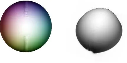
Figure 5: Surface normals and depth estimated from the polarisation image shown in Fig. 2 (and its right-illuminated counterpart). Surface normals are encoded by colour (azimuth) and saturation (zenith).
object. The resulting image is shown in Fig. 3, as also discussed in Section 2.
The specular inter-reflection can only just be seen in the intensity image, yet
the 90◦ phase shift and increased degree of polarisation make it clear in those
365
two components of the polarisation image.
The results of applying the surface normal estimation algorithm to the
po-larisation images shown in Figs. 2 and 3 are shown in Figs. 5 and 6,
respec-tively. The results are qualitatively good although the region of interpolation
(described in Section 3.3) near the top-centre and bottom-centre of the normal
370
maps is clearly apparent. Note that the data has been cropped here so only the
object itself is being integrated.
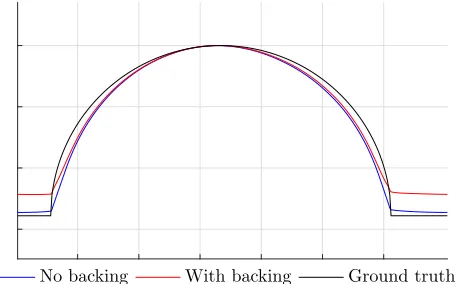
Fig. 7 shows a comparison of the profile of the reconstructions from Figs. 5
and 6 to ground truth data. To aid comparison, the profiles are aligned such
that the tops of each curve are touching. Very similar results were found for
375
pink and yellow balls, while blue and green results were slightly poorer due to
their lower brightness causing higher noise levels.
In order to optimise the surface normal estimates with regards to the light
source separation, both simulated and real-world data were analysed for varying
light source angles. For the simulated data, images were generated assuming no
380
inter-reflections/specularities were present and a range of illumination angles,
Figure 6: Surface normals and depth estimated from the polarisation image shown in Fig. 3 (and its right-illuminated counterpart). Surface normals are encoded by colour (azimuth) and saturation (zenith).
No backing With backing Ground truth
[image:24.612.194.422.445.587.2]5 10 15 20 25
Source angle (deg)
0 1 2 3 4 5
ε
(d
eg
)
[image:25.612.209.389.131.287.2]0 0.005 0.01 0.015
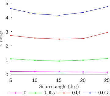
Figure 8: Surface normal errors using synthetic data with varying levels of Gaussian noise added (standard deviations shown in legend).
ranging from 0 (no noise) to 0.015 (typical for the camera settings used). The
results are shown in Fig. 8, where the performance metric used is the median
angular error,ε, between the method and ground truth. This metric has been
385
chosen since the more obvious choice of height residuals would also be assessing
the integration method used, which is not the contribution of the current paper.
The results to the analysis of simulated data show the following:
• The surface normals are not perfectly estimated even with no noise present
as a result of small surface regions being interpolated over. There may
390
also be some edge-effects degrading results slightly.
• There is relatively little variation in performance with illumination angle
for most noise levels.
• There is an optimum illumination angle of about 15◦ for higher noise
levels. This is due to the fact that (1) at very small angles the difference
395
between intensity images is very small which is poor conditioning for PS,
and (2) at large angles major areas of shadow are present.
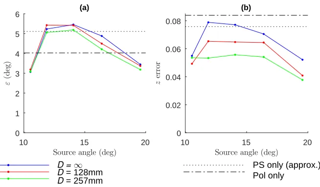
Experimental results for varying the illumination angle are shown in Fig. 9.
10 15 20 Source angle (deg) 0 1 2 3 4 5 6 ε (d eg ) (a)
10 15 20
Source angle (deg) 0 0.02 0.04 0.06 0.08 z er ro r (b)
D = ∞
D = 128mm
D = 257mm
PS only (approx.) Pol only
Figure 9: (a) Angular errors and (b) height errors for the white snooker ball with a white board at various distances behind the ball,D. Height values are in units such that a value of 1 corresponds to a distance of one radius. Best case results for PS-only and polarisation-only are also indicated.
the focus here is on the former due to reasons already mentioned.
Unsurpris-400
ingly, the magnitudes of the errors are slightly higher than for simulated data
for most cases. Surprisingly however, the trend towards an optimum separation
is reversed for the real data. It is not entirely clear why this should be the case
but repeated experiments have yielded similar trends. It was therefore decided
to use 20◦ illumination angles for the remainder of the research (higher values
405
than this were neither practical for the experimental rig being used nor for most
real-world applications).
Fig. 9 also shows results with the white board re-introduced at several
dis-tances and the baseline results for standard photometric stereo and single-source
polarisation. The results with the board present show a strong performance by
410
the method at overcoming specular inter-reflections, which is one of the key
strengths of the method. Indeed, there is evidence that in some cases the
recon-structions may be even better when strong specular behaviour is present. For
[image:26.612.143.470.121.312.2]that gave the best surface normal estimates for that method (which was
exper-415
imentally determined to be 25◦). For the single-source polarisation baseline, a
single polarisation image was used with the illumination source as close to the
camera as possible (βL =βR≈5◦ in practice) in order to minimise shadowed
regions. Regions of the image were manually selected in order to disambiguate
the azimuth angles and the zenith angles were calculated according to the Wolff
420
diffuse reflection model with a refractive index of 1.5 [7]. At first sight, the
baseline polarisation method appears comparable to the novel method, but it
is reiterated that the novel method is superior as it does not require manual
disambiguation nor knowledge of refractive index.
For the case with no board present behind the ball, a test on partially
sim-425
ulated data was conducted in order to analyse the relative effect of the PS and
polarisation elements of the method. Average angular errors for (1) entirely
real; (2) simulated polarisation (φandρ); and (3) simulated intensity (I) data
were: 7.6◦, 6.4◦and 2.9◦respectively. This is rather striking as it shows the PS
component has by far the largest associated error. This is presumably due to
430
the resilience of polarisation phase data against reflectance properties compared
to PS and the lesser need for carefully positioned light sources. It should be
noted however, that such a breakdown of experimental error may change for
certain target objects, such as where large areas of the surface have very low
degree of polarisation.
435
These areas of low degree of polarisation have associated high noise levels
and may be a potential weakness of the method. Results so far in this paper
overcame this in a rather expensive manner by capturing 100 images in very
rapid succession for each of the four polariser angles. The effects of using fewer
images is illustrated by Fig. 10 which shows the estimated surface normal (y
-440
andz-components only for compactness) using 1, 5, 20 and 100 images. At first
sight, the quality of results is poor when only few images are used. However,
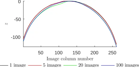
the increased noise has a relatively low impact on surface height reconstruction,
as shown in the Fig. 11. This is due to the facts that (1) the Frankot-Chellappa
surface integrator is smoothing over the noise, and (2) the higher noise regions
-1 -0.5 0 0.5 1 Distance from axis -1
-0.5 0 0.5 1
Ny
-1 -0.5 0 0.5 1
Distance from axis 0.2
0.4 0.6 0.8 1
Nz
[image:28.612.144.464.127.277.2]1 image 5 images 20 images 100 images
Figure 10: Comparison between surface normal estimates for varying number of images per polariser angle for a cross-section of the snooker ball.
50 100 150 200 250
Image column number -100
-50 0
z
1 image 5 images 20 images 100 images
Figure 11: Comparison between surface depth estimates for varying number of images per polariser angle for a cross-section of the snooker ball.
correspond to areas of low zenith angle which have smaller effects on the
inte-gration than those of larger zenith angle.
4.2. Other objects
Surface normal estimates for two cylinders are shown in Fig. 12. For this
case, the cylinders are both porcelain: one pure white and one multicoloured,
450
as shown in Fig. 13. The results clearly show a close match to theory; with the
main discrepancy being at the occluding contours. For the case shown, the axes
of the cylinders were oriented parallel to thex-axis (see Fig. 1). Unfortunately,
the method completely fails for the case where the cylinder axis is parallel to
y-axis. This is due to the fact that all pixels on the surface in such cases appear
[image:28.612.189.421.322.436.2]-1 -0.5 0 0.5 1 Distance from axis -1
-0.5 0 0.5 1
Ny
-1 -0.5 0 0.5 1
Distance from axis 0
0.2 0.4 0.6 0.8 1
Nz
[image:29.612.138.471.128.282.2] [image:29.612.267.343.327.424.2]Ground truth White cylinder Multicolour cylnder
Figure 12: Comparison between surface normal estimates and ground truth for a white porce-lain and multicoloured porceporce-lain cylinder.
Figure 13: Photograph of the multicoloured cylinder used for Fig. 12.
equally bright from each light source, making seed selection and region growing
nearly impossible: a clear weakness of the method which will be addressed in
future work.
Tests on objects of more complicated geometry are shown in Figs. 14 and
15. The general geometries of the fruits in Fig. 14 have clearly been reproduced,
460
albeit with over-smoothing in places. The model dinosaur in Fig. 15 also has
reasonable shape, despite a few areas of incorrect disambiguation on the foot
and head. It is hoped that such issues might be resolved in future work by
Figure 14: Surface reconstructions of an apple and lemon.
[image:30.612.201.406.475.587.2]4.3. An alternative integrator
465
The choice of the Frankot-Chellappa integration method for conversion from
normals to depth was made since (1) it is well-established in the field and (2) it
operates at high speed (much less than one second to reconstruct a VGA frame).
However, the method is not very effective in certain circumstances. The most
known of its weaknesses is its tendency to over-smooth surfaces as a result of
470
its basis functions being unsuited to discontinuities.
Another weakness, which is more specific to the method of this paper,
re-lates to the fact that the integrator applies equal weighting to all points on the
surface. While this is sensible for most reconstruction methods, the approach
here may benefit from weighting certain pixels more than others. Specifically,
475
it is beneficial to give a higher weight to pixels of higher degree of polarisation
since those are less prone to noise/distortion.
An alternative integrator that is much less affected by discontinuities and
allows for variable pixel weighting is that of the M-estimator [34]. Fig. 16
demonstrates the advantage of the M-Estimator approach using the underside
480
of a porcelain bowl as a test object. The figure first shows the result of using
the Frankot-Chellappa method. The result is highly distorted at the base of the
bowl since the degree of polarisation is very low here over a wide area. In an
effort to mitigate these effects, the M-Estimator was used with the weight set
to zero wherever the degree of polarisation is less than 1%. As shown in the
485
figure, this significantly improves results for most of the surface1. The obvious
disadvantage of this approach was that the integration took much longer (≈40 s
compared to≈0.1 s).
5. Conclusion
Results in this paper demonstrate the potential for use of polarisation
in-490
formation for scene understanding in the presence of both diffuse reflection
Figure 16: Reconstructions of the underside of a porcelain bowl, including the side view. The left reconstructions were based on the Frankot-Chellappa method, while those to the right use the M-Estimator.
and specular inter-reflections. The results show reconstruction quality that is
improved or comparable with the baseline methods while needing only two
il-lumination sources, which is competitive to many other methods in the field.
At present, the data is captured using a rotating polariser and switching light
495
sources meaning the data takes several seconds to capture. As stated in Section
2 however, the method can be applied to data captured from a polarisation
camera such as the POLKA. This means that the only significant limitation in
capture time relates to the light source switching, which has easily been shown
to operate in the order of milliseconds [5]. The processing time for this method
500
is of the order five seconds at VGA resolution on an average personal computer.
The method has clearly demonstrated the use of polarisation information
to reduce the number of light sources needed for photometric stereo to two.
Unlike with many alternative methods in polarisation vision, this advantage
does not come at the expense of needing to know a refractive index or
mak-505
ing strong assumptions on reflectance properties. One major weakness of many
PS methods is that of shadowing. While the novel method still suffers from
reduced information at shadowed regions; only the zenith angle is affected. It
is therefore predicted that the estimated azimuth angles for such regions may
be combined with intensity information from one source only to fully recover
510
shadowed surfaces in follow-on work. The dependence of the method on the
reflectance properties of the surface is also deemed superior to many PS
reflectance parameters. That said, it is acknowledged that the proposed
ap-proach is still somewhat affected by reflectance properties due to the use of (8)
515
for thez-component of the normal.
One limitation that should be addressed in future work relates to the open
question of how to recover the geometry of an entire scene (as opposed to a
single object). It may be that optimisation of seed point generation and
weight-ing inter-object pixels in the integrator may reduce this limitation. Another
520
limitation relates to the complications caused by very rough surfaces. The main
problem caused by roughness for many polarisation-based methods is the
de-polarising effect of microscopic inter-reflections on the surface. This typically
has a direct degrading effect on the reconstruction because the zenith angle is
inherently dependent on degree of polarisation. For the method proposed in
525
this paper however, the zenith angle is entirely determined by PS, diminishing
the effects of roughness. Nevertheless, the increased noise present due to lower
degrees of polarisation from rough surfaces will still clearly impact results of the
method to an extent.
References 530
[1] M. Z. Brown, G. D. Hager, Advances in computational stereo, IEEE Trans.
Patt. Anal. Mach. Intell. 25 (2003) 993–1008.
[2] S. Foix, G. Aleny`a, Lock-in time-of-flight (ToF) cameras: A survey, IEEE
Sensors J. 11 (2011) 1917–1926.
[3] J. D. Durou, M. Falcone, M. Sagnona, Numerical methods for
shape-from-535
shading: A new survey with benchmarks, Comp. Vis. Im. Understanding
109 (2008) 22–43.
[4] P. N. Belhumeur, D. J. Kriegman, A. L. Yuille, The bas-relief ambiguity,
Intl. J. Comp. Vis. 35 (1999) 33–44.
[5] M. F. Hansen, G. A. Atkinson, L. N. Smith, M. L. Smith, 3D face
structions from photometric stereo using near infrared and visible light,
Comp. Vis. Im. Understanding 114 (2010) 942–951.
[6] W. Zhang, M. L. Smith, L. N. Smith, A. Farooq, Gender recognition from
facial images: two or three dimensions?, J. Opt. Soc. Am. A 33 (2016)
333–344.
545
[7] L. B. Wolff, T. E. Boult, Constraining object features using a polarisation
reflectance model, IEEE Trans. Patt. Anal. Mach. Intell. 13 (1991) 635–657.
[8] E. Hecht, Optics, 3rd Edition, Addison Wesley Longman, 1998.
[9] M. Saito, Y. Sato, K. Ikeuchi, H. Kashiwagi, Measurement of surface
ori-entations of transparent objects using polarization in highlight, in: Proc.
550
CVPR, Vol. 1, 1999, pp. 381–386.
[10] D. Miyazaki, M. Kagesawa, K. Ikeuchi, Transparent surface modelling from
a pair of polarization images, IEEE Trans. Patt. Anal. Mach. Intell. 26
(2004) 73–82.
[11] G. A. Atkinson, E. R. Hancock, Shape estimation using polarization and
555
shading from two views, IEEE Trans. Patt. Anal. Mach. Intell. 29 (2007)
2001–2017.
[12] K. Berger, R. Voorhies, L. Matthies, Incorporating polarization in stereo
vision-based 3D perception of non-Lambertian scenes, in: Proc. SPIE, Vol.
9837, 2016.
560
[13] V. Taamazyan, A. Kadambi, R. Raskar, Shape from mixed polarization,
arXiv preprint: 1605.02066.
[14] D. Miyazaki, R. T. Tan, K. Hara, K. Ikeuchi, Polarization-based inverse
rendering from a single view, in: Proc. ICCV, Vol. 2, 2003, pp. 982–987.
[15] O. Drbohlav, R. ˇS´ara, Unambiguous determination of shape from
pho-565
tometric stereo with unknown light sources, in: Proc. ICCV, 2001, pp.
[16] O. Drbohlav, R. ˇS´ara, Specularities reduce ambiguity of uncalibrated
pho-tometric stereo, in: Proc. ECCV, 2002, pp. 46–62.
[17] G. A. Atkinson, E. R. Hancock, Two-dimensional BRDF estimation from
570
polarisation, Comp. Vis. Im. Understanding 111 (2008) 126–141.
[18] T. Ngo, H. Nagahara, R. Taniguchi, Shape and light directions from shading
and polarization, in: In Proc. CVPR, 2015, pp. 2310–2318.
[19] N. M. Garcia, I. de Erausquin, C. Edmiston, V. Gruev, Surface normal
re-construction using circularly polarized light, Opt. Express 23 (2015) 14391–
575
14406.
[20] O. Morel, C. Stolz, F. Meriaudeau, P. Gorria, Active lighting applied to
three-dimensional reconstruction of specular metallic surfaces by
polariza-tion imaging, Applied Optics 45 (2006) 4062–4068.
[21] W. Smith, R. Ramamoorthi, S. Tozza, Linear depth estimation from an
580
uncalibrated, monocular polarisation image, in: In Proc. ECCV, 2016, pp.
109–125.
[22] S. Rahmann, N. Canterakis, Reconstruction of specular surfaces using
po-larization imaging, in: Proc. CVPR, 2001, pp. 149–155.
[23] S. Rahmann, Reconstruction of quadrics from two polarization views, in:
585
Proc. IbPRIA, 2003, pp. 810–820.
[24] C. P. Huynh, A. Robles-Kelly, E. Hancock, Shape and refractive index
recovery from single-view polarisation images, in: Proc. CVPR, 2010, pp.
1229–1236.
[25] A. Kadambi, V. Taamazyan, B. Shi, R. Raskar, Polarized 3D: High-quality
590
depth sensing with polarization cues, in: Proc. ICCV, 2015.
[26] G. A. Atkinson, E. R. Hancock, Recovery of surface orientation from diffuse
[27] L. B. Wolff, Diffuse-reflectance model for smooth dielectric surfaces, J. Opt.
Soc. Am. A 11 (1994) 2956–2968.
595
[28] Fraunhofer Institute for Integrated Circuits, http://
www.iis.fraunhofer.de/en/ff/bsy/tech/kameratechnik/
polarisationskamera.html, [Accessed: 1 March 2017].
[29] W. Burger, M. J. Burge, Principles of Digital Image Processing:
Funda-mental Techniques, Springer, 2010.
600
[30] N. Karpel, Y. Schechner, Portable polarimetric underwater imaging system
with a linear response, in: Proc. SPIE, Vol. 5432, 2004.
[31] R. J. Woodham, Photometric method for determining surface orientation
from multiple images, Optical Engineering 19 (1980) 139–144.
[32] R. F. Saracchini, J. Stolfi, H. C. G. Leit˜ao, G. A. Atkinson, M. L. Smith,
605
A robust multi-scale integration method to obtain the depth from gradient
maps, Comp. Vis. Im. Understanding 116 (2012) 882–895.
[33] R. T. Frankot, R. Chellappa, A method for enforcing integrability in shape
from shading algorithms, IEEE Trans. Patt. Anal. Mach. Intell. 10 (1988)
439–451.
610
[34] A. Agrawal, R. Raskar, R. Chellappa, What is the range of surface
LaTeX Souce Files