Evaluation of different soil water potential by field capacity threshold in combination with a triggered irrigation module

Evaluation of Different Soil Water Potential by Field

Capacity Threshold in Combination with a Triggered

Irrigation Module

Monika MARKOVIĆ

_{, Vilim FILIPOVIĆ}

_{, Tarzan LEGOVIĆ}

_{, Marko JOSIPOVIĆ}

and Vjekoslav TADIĆ

1_{Faculty of Agriculture, University of J.J. Strossmayer in Osijek, Osijek, Republic of Croatia;} 2_{Department of Soil Amelioration, Faculty of Agriculture, University of Zagreb, Zagreb,} Republic of Croatia; 3_{Ruđer Bošković Institute, Zagreb, Republic of Croatia;} 4_Agricultural

Institute in Osijek, Osijek, Republic of Croatia

Abstract

Marković M., Filipović V., Legović T., Josipović M., Tadić V. (2015): Evaluation of different soil water potential by field capacity threshold in combination with a triggered irrigation module. Soil & Water Res., 10: 164–171.

Irrigation efficiency improvement requires optimization of its parameters like irrigation scheduling, threshold and amount of water usage. If these parameters are not satisfactorily optimized, negative consequences for the plant-soil system can occur with decreased yield and hence economic viability of the agricultural production. Numeri-cal modelling represents an efficient, i.e. simple and fast method for optimizing and testing different irrigation scenarios. In this study HYDRUS-1D model assuming single- and dual-porosity systems was used to evaluate a triggered irrigation module for irrigation scheduling in maize/soybean cropping trials. Irrigation treatment con-sisted of two irrigation regimes (A2 = 60–100% field capacity (FC) and A3 = 80–100% FC) and control plot (A1) without irrigation. The model showed a very good fit to the measured data with satisfactory model efficiency values of 0.77, 0.69, and 0.93 (single-porosity model) and 0.84, 0.67, and 0.92 (dual-porosity model) for A1, A2, and A3 plots, respectively. The single-porosity model gave a slightly better fit in the irrigated plots while the dual-porosity model gave better performance in the control plot. This inconsistency between the two approaches is due to the manual irrigation triggering and uncertainty in field data timing collection. Using the triggered irrigation module provided more irrigation events during maize and soybean crop rotation and consequently increased cumulative amounts of irrigated water. However, that increase resulted in more water available in the root zone during high evapotranspiration period. The HYDRUS code can be used to optimize irrigation threshold values further by as-suming different scenarios (e.g. different irrigation threshold or scheduling) or a different crop.

Keywords: field water capacity; dual-porosity model; HYDRUS-1D; numerical modelling; single-porosity model; trig-gered irrigation

Increasing worldwide water shortages and costs of irrigation are leading to an emphasis on the develop-ment of irrigation methods that minimize water use efficiency (Jones 2004). Water use efficiency can be improved by irrigation scheduling which saves water and energy. Irrigation scheduling is based on monitoring indicators that determine the need for irrigation based on type of plant, soil, or climate

(FC), i.e. of the upper limit of water storage in soil. Soil moisture content at FC is the amount of water retained in the soil after the drainage due to gravita-tional forces. Usually the soil is considered to be at FC when the water potential in the soil is at –33 kPa. The soil FC is mostly determined using the pressure plate measurement. The amount of water applied by irrigation needs to replace soil moisture depletion, yet the excessive amount of water leads to nutrient leaching, pollution of aquifers, and financial losses as well. Although soil moisture monitoring can be effectively used for irrigation scheduling purpose, this process is labour intensive and time consuming and it may not be economically viable (George et al. 2000).

A number of numerical models have been developed and used in irrigation research like SOWATCHM (Dudley & Hanks 1991) or ENVIRO-GRO (Pang & Letey 1998). According to Dudley et al. (2008), the HYDRUS model represents the most frequently used and the most accessible simulation tool for water and solutes dynamics in soil. HYDRUS-2D model was successfully used for modelling water flow in drip irrigation systems (Lazarovitch et al. 2005; Mubarak et al. 2009) and for evaluating the effects of soil texture and gravel cavity dimension in a sub-surface drip irrigation system (Ben Gal et al. 2004). Kodešová and Brodský (2006) used the simulation model CGMS-WOFOST to simulate water balance in the root zone. The authors compared the obtained results to the Richards’ equation based HYDRUS-1D model and found lower values of relative water con-tent obtained using CGMS-WOFOST mostly due to higher retention ability of HYDRUS-1D. Dabach et al. (2013) compared field experimental data to results from modelling with HYDRUS-2D/3D and found good agreement between irrigation events and pressure heads with experimental data. Trig-gered drip irrigation, controlled by loop irrigation system linked to tensiometers, was used at two soil types. The main aim of this research was to evaluate the triggered irrigation module in HYDRUS-1D for irrigation scheduling using manually collected field pressure head measurement based on the FC (60 and 80%) in maize/soybean cropping trials.

MATERIAL AND METHODS

Field experiment. Field data were collected at the experimental field of the Agricultural Institute in Osijek, eastern Croatia (45°32''N and 18°44''E,

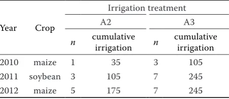
altitude 90 m) within 2010–2012. Maize (Zea mays L.) was cropped in 2010 and 2012, while soybean (Glycine max L.) was grown during 2011. Two irrigation treat-ments and a control were used in each year. Trials included control plot without irrigation (A1), irrigation at 60% of FC (A2) and at 80% of FC (A3). Total size of each irrigation plot was 235 m2_{. Plots were irrigated} using a travelling gun sprinkler irrigation system. The system operated at the average speed of 15 m/h and provided 35 mm of irrigation water (1.5 l/min) with manual handling. Irrigation scheduling was based on pressure head measuring by Watermark sensors (Ir-rometer, Riverside, USA) installed at each irrigation plot. The sensors were set up at two depths (15–20 cm and 25–30 cm) after the maize/soybean sowing and were kept in soil until harvest time. Watermark sensors measure soil water tension with 0–200 centibar range, where 0 represents 100% of FC and 200 represents dry soil. Irrigation in A2 plot was performed at 60% of FC which corresponds to a value of –815 cm. In A3 plot the irrigation threshold was at 80% of FC, i.e. –509 cm of pressure head. At each year and irrigation treatment, the amount of water applied per one irrigation event was 35 mm. Total amounts of irrigation water applied for each growing season are presented in Table 1. Daily weather data were obtained from the agro-climatic sta-tion in Osijek, located approximately 10 km from the field experiment. The readings included: rainfall, air humidity, wind speed, daily minimum and maximum air temperatures, and solar radiation.

Soil parameters. The soil type classified at the experimental site was Luvic Stagnic Phaeozem Siltic (horizons: Ap-Bt-Bg-C). Soil samples were taken with an auger and the main physical and chemical analyses were conducted. The particle size distribution (frac-tions of sand, silt, and clay) was determined using the pipette method (Gee & Or 2002). An undisturbed soil sample of 100 cm3 _{was used to determine bulk density}

Table 1. Amount of irrigation water applied per each tre-atment (A2 and A3) during 2010–2012 (in mm)

Year Crop

Irrigation treatment

A2 A3

n cumulative _irrigation n cumulative _irrigation

2010 maize 1 35 3 105

2011 soybean 3 105 7 245

2012 maize 5 175 7 245

A2 = 60% field capacity (FC); A3 = 80% FC; n = No. of

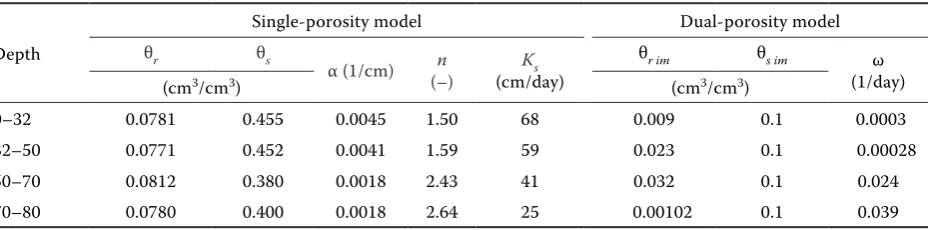
and soil hydraulic properties in each layer (e.g. soil water retention and hydraulic conductivity curves). Saturated hydraulic conductivity K_s was determined using the constant head method (Klute & Dirksen 1986). Saturated water content θ_s was measured using ISO 11274:1998 (i.e. sandbox method). The points of the soil water retention curve were measured using a pressure plate apparatus with applied pressures of 3, 33, 625, and 1500 kPa, consecutively. The soil hydraulic parameters used in the modelling study are presented in Table 2.

Pressure head simulations using single- and dual-porosity models. Measured soil pressure heads were simulated using the modified form of the Richards’ equation (Šimůnek et al. 2008) for water move-ment in unsaturated soils under one dimensional uniform flow:

(1)

where:

θ – volumetric water content (cm3_/cm3₎ h – soil water pressure head (cm)

t – time (days)

z – soil depth (cm)

S – sink term for root water uptake

Sink term was modelled using Feddes equation (Feddes et al. 1978):

S(h) = α(h)S_p (2)

where:

α(h) – water stress response function, which varies between 0 and 1

S_p – potential root water uptake rate (1/day)

The unsaturated hydraulic conductivity K (cm per day), as a function of h, is given in the van Ge-nuchten’s equation (i.e. single-porosity model) (Van Genuchten 1980):

_{for h < 0 (3)}

θ(h) = θ_s for h ≥ 0

(4)

(5)

;n>1 (6)

where:

θ(h) – volumetric water content (cm3_/cm3₎

K(h) – unsaturated hydraulic conductivity (cm/day)

θ_r, θ_s – residual and saturated water contents (cm3_/cm3₎ S_e – effective saturation

K_S – saturated hydraulic conductivity (cm/day) α – inverse of air-entry value or bubbling pressure

(1/day)

n – pore size distribution index

m − empirical shape parameter in the soil water retention function (−)

l – pore connectivity parameter

The pore connectivity parameter (l = 0.5) represents an average value for many soil types (Mualem 1976). Values of α and n were optimized by inverse modelling, i.e. by fitting pressure head measured at soil profile and lysimeter outflow installed at a 80 cm depth using the van Genuchten-Mualem single-porosity model in HYDRUS-1D. The initial values of α, n, and θ_r were estimated from measured water retention data using RETC (Van Genuchten et al. 1991).

In order to consider the possibility of preferential flow effect in the field that could be expected in regions of enhanced flux in such a way that a small fraction of media (e.g. wormholes, root holes, cracks or channels) participates in a large volume of the flow, we have additionally performed simulations

Table 2. Van Genuchten soil physical parameters used in single- and dual-porosity models

Depth

Single-porosity model Dual-porosity model

θr θs

α (1/cm) _(–)n Ks

(cm/day)

θr im θs im ω

(1/day)

(cm3_/cm3_{) (cm}3_/cm3₎

0–32 0.0781 0.455 0.0045 1.50 68 0.009 0.1 0.0003

32–50 0.0771 0.452 0.0041 1.59 59 0.023 0.1 0.00028

50–70 0.0812 0.380 0.0018 2.43 41 0.032 0.1 0.024

70–80 0.0780 0.400 0.0018 2.64 25 0.00102 0.1 0.039

∂θ = ∂

[

(

)]

∂θ ∂z ∂z

θ(h) = θ_r + θs − θr

(1 + |αh|n)m

K(h) = K_SS_el_{(1 − (1 −S} e 1/m₎m₎2

S_e = θ − θr

θs−θr

m = 1 − 1

using dual-porosity assumption. The dual-porosity formulation for water flow as used in HYDRUS-1D is based on a mixed formulation, which uses the Richards’ equation (1) to describe water flow in the fractures (macropores), and a simple mass balance equation to describe moisture dynamics in the matrix as follows (Šimůnek et al. 2003):

(7)

(8)

where:

m, im – mobile and immobile water regions θ = θ_m+θ_im – volumetric water content (cm3_/cm3₎ S_im, S_m – sink terms (root water uptake) for both

regions (1/day)

Γ_w – transfer rate for water exchange between macropores and matrix (1/day)

The mass transfer rate, Γ_w, for water between the fracture and matrix regions in several dual-porosity studies has been assumed to be proportional to the difference in effective water contents of the two regions using the first-order rate equation:

(9)

where:

θ_im – matrix water content

ω – first-order rate coefficient (1/day)

S_em

,

–

To obtain necessary parameters for the dual-po-rosity modelling, three parameters (θ_m, θ_im,and ω) for each soil layer (12 parameters in total) were optimized by inverse simulations using a similar procedure as for the single-porosity model with the assumption that the parameters used in the single-porosity model were accurately predicted.

Initial and boundary conditions. One-dimensional flow in the vertical direction was assumed for which HYDRUS-1D was sufficient. The profile was set down to 80 cm depth, since soil properties were measured in that depth range and tensiometers were installed to 30 cm depth. One average measurement of soil pressure head was used at each plot for results comparison (two sensors were installed). The initial condition for water content was set as a hydrostatic pressure head distribution with −100 cm at the bot-tom of soil profile at the beginning of 2010. The time

period for simulations was from January 1, 2010 until December 31, 2012, split into three separate simulations (there is no option for crop rotation in HYDRUS-1D, therefore each crop vegetation period, i.e. maize, soybean, maize, was simulated separately) which were connected sequentially by assigning the final pressure head distribution from the preceding simulation as an initial condition for the next one. Free drainage boundary condition was assigned to the bottom of the flow domain and an atmospheric boundary condition was assigned to the soil surface. The atmospheric boundary condition at the surface was described using meteorological input data (i.e. rainfall and the evapotranspiration amounts) includ-ing irrigated water. HYDRUS-1D uses a module in which irrigation can be triggered when a certain pressure head is reached, at selected observation node, at a user-specified irrigation rate and duration. The triggered irrigation module was confronted with manual field irrigation triggering based on pressure head measurement. The irrigation in the model was triggered at –815 cm (60% FC) and –509 (80% FC) at the soil surface, with a duration of 20 min and a rate of 35 mm. The model of Feddes et al. (1978) was used for root water uptake rates evaluation which is assigned according to the pressure potential (h) of the soil water. Essentially, a plant-dependent, optimum uptake range exists between the two h values while the uptake rate decreases linearly to zero when h is above or below this range. These values were taken from HYDRUS database i.e. set for maize and alfalfa (the parameters for soybean were not available in the model). Crop growth parameters (crop height and rooting depth) were estimated at the field site and were used as input parameters for HYDRUS-1D for potential evaporation and transpiration rates cal-culation according to Penman–Monteith approach (Monteith 1981). Model efficiency coefficient E (Nash & Sutcliffe 1970) and Pearson’s coefficient of determination (R2_{) were used to assess the level} of agreement between predicted and observed pres-sure head data.

RESULTS AND DISCUSSION

Prior to Watermark sensor installation, in-soil cali-bration of the sensor was performed. The calicali-bration was based on gravimetric water content measurement on undisturbed soil samples taken at the site (May, 2010). The calibration was performed successfully and sensors were installed in the soil profile on each

∂θm = ∂

[

(

)]

∂t ∂z ∂z

∂θim _{= −S} im + Γw

∂t

Γ_w = ∂θim = ω[_S e m _{− S}

eim]

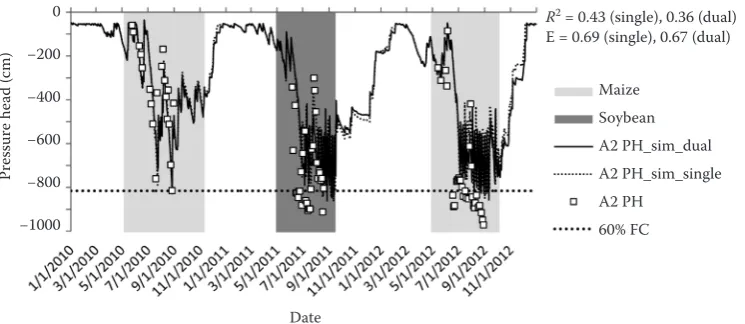
plot during 2010–2012. Simulations were performed for the same period using the procedure explained above. The changes in observed and simulated pres-sure head values were similar throughout the moni-toring period. Simulated data followed the observed data and showed very good agreement in all plots. The model efficiency coefficients were 0.77, 0.69, and 0.93 (single-porosity model) and 0.84, 0.67, and 0.92 (dual-porosity model) for A1, A2, and A3 plots, respectively (Figures 1–3).

A noticeable increase in model efficiency and fitting can be seen in A1 control plot using the dual-poros-ity assumption. These results indicate the possible presence of preferential flow events during the re-search period. However, in other two irrigated plots (A2, A3) the single-porosity model derived slightly better results. Since the model triggers the irriga-tion exactly at the pressure head values of –815 cm (A2) and –509 cm (A3) and does not allow the

pres-sure drop below the selected thresholds, at certain point the simulated data does not fit the observed ones below those pressure head points. The main reason for this observed discrepancy is the manual irrigation triggering and pressure head monitoring in the field, thus we observed values lower than the threshold values (especially in A2 plot, Figure 2) due to a delay in the irrigation/measurement procedure. In A1 control plot one notices a very large decrease of pressure head values, especially during 2011 with a decrease of up to –9200 cm. In that specific year, there was only 422 mm of rainfall which is by 25% less than was the 30-year average (1961–1990 = 566.2 mm) on that particular location. The largest drop in pressure head values was recorded at the reproductive stage which can significantly reduce yield of summer crops (Barnabás et al. 2008). Since pressure head and soil water content distributions in the root zone are key factors that affect biomass

Figure 1. Observed (symbols) vs simulated (line) pressure head distribution at a 25 cm depth during 2010–2012 for A1 scenario (no irrigation); E − model efficiency coefficient

Figure 2. Observed (symbols) vs simulated (line) pressure head distribution at a 25 cm depth during 2010–2012 for A2 scenario (60% of field capacity); E − model efficiency coefficient

Pr

essur

e he

ad (

cm)

Date 0

−2000

−4000

−6000

−8000

−10 000

R2 _{= 0.65 (single), 0.71 (dual)} E = 0.77 (single), 0.84 (dual)

Maize Soybean A1 PH_sim_dual A1 PH_sim_single A1 PH

Pr

essur

e he

ad (

cm)

Date 0

−200

−400

−600

−800

−1000

R2 _{= 0.43 (single), 0.36 (dual)} E = 0.69 (single), 0.67 (dual)

Maize Soybean A2 PH_sim_dual A2 PH_sim_single A2 PH

production (Shani et al. 2004), it is crucial to es-tablish a favourable water balance in the root zone. At the A2 plot triggered irrigation, the model was set to start irrigation when the pressure head value dropped below –815 cm resulting in more wetting of the soil during the whole period, thus providing more available water for crops. Figure 2 shows clearly that observed values of pressure head were below the selected threshold values. This can be seen during 2011 and 2012 in the middle of the summer/vegeta-tion period since manual irrigasummer/vegeta-tion was probably not that accurate and irrigation was performed with some delay as stated before. On the other hand, the model automatically triggered irrigation when the pressure head reached the threshold value and this “delay” effect was absent in the performed simulations. The same is true for A3 plot with a different thresh-old value used (–509 cm); therefore the irrigation was performed on a different schedule than before

resulting in larger amount of cumulative irrigation (Table 1). However, to maintain the pressure head at two selected threshold values (i.e. 60% and 80% FC), more irrigation events need to be applied. Dabach et al. (2013) used similar approach by evaluating HYDRUS-2D/3D in terms of fitting soil water

infil-Figure 3. Observed (symbols) vs simulated (line) pressure head distribution at a 25 cm depth during 2010–2012 for A3 scenario (80% of field capacity); E − model efficiency coefficient

Table 3. Simulated cumulative amounts of irrigation water applied during 2010–2012

Year Treatment No. of events Cumulative irrigation _amount

2010 A2_A3 2_{3 105}70

2011 A2_A3 12₁₃ 420₄₅₅

2012 A2 13 455

A3 14 490

A2 − 60% field capacity (FC); A3 − 80% FC Date

0

−100

−200

−300

−400

−500

−600

R2 _{= 0.59 (single), 0.58 (dual)} E = 0.93 (single), 0.92 (dual)

Maize Soybean A3 PH_sim_dual A3 PH_sim_single A3 PH

80% FC

Pr

essur

e he

ad (

cm)

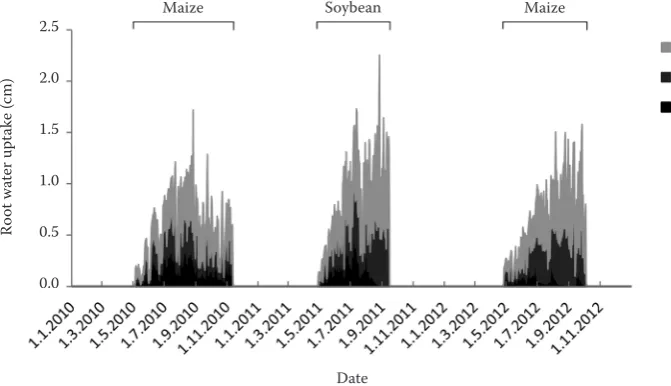
Figure 4. Simulated root water uptake in A1, A2, and A3 tre-atments during 2010–2012

A3_Root uptake A2_Root uptake A1_Root uptake

Date

Ro

ot w

at

er upt

ak

e (

cm)

2.5

2.0

1.5

1.0

0.5

0.0

tration, redistribution, and root water uptake under the drip irrigation in sandy soils. Simulated soil pressure heads at an observation point, for differ-ent boundary and initial conditions, were found to be in a good agreement with experimental data and triggered the same number of irrigation pulses as the experimental automated systems. Since in our field experiment we had manual triggering with surface sprinkler irrigation, which is not as precise as the drip irrigation in terms of equal water distribution, the simulations provided more irrigation events, i.e. more water to maintain the desired soil water con-tent. For all irrigation events, HYDRUS simulations showed simultaneous increases in pressure head and soil water content after irrigation. In addition, they present instantaneous responses during irrigation water redistribution phases. For most times and for all treatments, the manually measured pressure heads are very similar to the modelled ones. Table 3 shows the simulated cumulative irrigation that was applied to maintain the desired water balance in the profile. One can see that more irrigation needs to be applied in order to fulfill these requirements and to keep the pressure head not to drop below 60% and 80% of FC, respectively. Finally, root water uptake had very different values in each treatment (Figure 4), thus affecting the crop growth and consequently yield (data not shown). The cumulative values of root water uptake were 736, 1377, and 1392 mm for A1, A2, and A3 plots, respectively. These results clearly demonstrate the importance of irrigation in the period of year with high evapotranspiration values and low rainfall. Each irrigation regime needs a specific irrigation threshold to be able to supply appropriate amounts of water to plants. This can easily be ensured by using HYDRUS model assuming different scenarios.

CONCLUSIONS

HYDRUS-1D model using single- and dual-porosity assumption with triggered irrigation module was con-fronted with the field measurement of pressure heads using Watermark sensors in two irrigation treatments, A2 initiating irrigation at 60% of field capacity, A3 initiating irrigation at 80% of field capacity, and A1 which was used as a control plot without any irriga-tion applied. The model performed with satisfactory efficiency values of 0.77, 0.69, and 0.93 (single-porosity model) and 0.84, 0.67, and 0.92 (dual-porosity model) for A1, A2 and A3 plots, respectively. Using the

trig-gered irrigation module provides more irrigation events and, consequently, increased cumulative amounts of water requirements needed to maintain a desired water balance in the profile. However, that increase resulted in more water available in the root zone during a high evapotranspiration period. The HYDRUS code can be used to optimize irrigation threshold values for specific boundary conditions and different crop. The boundary conditions can be updated during the growing season and used to determine new irrigation thresholds to compensate for increasing root water uptake by plants when needed, and in a simple and effective way provide results which can satisfy crop water requirements.

References

Barnabás B., Jäger K., Fehér A. (2008): The effect of drought and heat stress on reproductive processes in cereals. Plant, Cell & Environment, 1: 11–38.

Ben Gal A., Lazarovitch N., Shani U. (2004): Subsurface Drip Irrigation in Gravel-filled Cavities. Vadose Zone Journal, 3: 1407–1413.

Dabach S., Lazarovitch N., Šimůnek J., Shani U. (2013): Numerical investigation of irrigation scheduling based on soil water status. Irrigation Science, 31: 27–36. Dudley L.M., Hanks R.J. (1991): Model SOWACH:

Soil-plant-atmosphere-salinity Management Model Users’ Manual. Utah Agricultural Experiment Station Research Report No. 140. Logan, Utah State University.

Dudley L.M., Ben-Gal A., Lazarovitch N. (2008): Drainage water use: biological, physical and technological consid-erations for system management. Journal of Environmen-tal Quality, 37: 25–35.

Feddes R.A., Kowalik P.J., Zaradny H. (1978): Simulation of Field Water Use and Crop Yield. New York, John Wiley & Sons.

Gee G.W., Or D. (2002): Particle size analysis. In: Methods of Soil Analysis: Part 4, Physical Methods. Madison, SSSA: 255–293.

George B.A., Shende S.A., Raghuwanshi N.S. (2000): De-veloping and testing of irrigation scheduling model. Ag-ricultural Water Management, 46: 121–136.

Heimovaara T.J., Bouten W. (1990): A computer-controlled 36-chanell time domain reflectrometry system for moni-toring soil water content. Water Resource Research, 26: 2311–2316.

Part 1, Physical and Mineralogical Methods. Agronomy Monograph No. 9. Madison, ASA-SSSA.

Kodešová R., Brodský L. (2006): Comparison of CGMS-WOFOST and HYDRUS-1D simulation results for one cell of CGMS-GRID50. Soil and Water Research, 2: 39–48. Lazarovitch N., Šimůnek J., Shani U. (2005): System depend-ent boundary conditions from water flow from subsurface source. Soil Science Society of American Journal, 69: 46–50.

Monteith J.L. (1981): Evaporation and surface temperature. Quarterly Journal of the Royal Meteorological Society, 107: 1–27.

Mualem Y. (1976): A new model for prediction of the hy-draulic conductivity of unsaturated porous media. Water Resources Research, 12: 513–522.

Mubarak I., Mailhol M.C., Angulo-Jaramillo R., Bouarfa S., Ruelle P. (2009): Effect of temporal variability in soil hydraulic properties on simulated water transfer under high-frequency drip irrigation. Agricultural Water Man-agement, 96: 1547–1559.

Nash J.E., Sutcliffe J.V.(1970): River flow forecasting through conceptualmodels. Part I. A discussion of principles. Journal of Hydrology, 10: 282–290.

Pang X.P., Letey J. (1998): Development and evaluation of ENVIROGRO, an integrated water, salinity, and nitrogen model. Soil Science Society of American Journal, 62: 1418–1427.

Shani U., Tsur Y., Zemel A. (2004): Optimal dynamic irriga-tion schemes. Optimal Control and Applicairriga-tion Methods, 25: 91–106.

Šimůnek J., Jarvis N.J., Van Genuchten M.T., Gärdenäs A. (2003): Review and comparison of models for describing non-equilibrium and preferential flow and transport in the vadose zone. Journal of Hydrology, 272: 14–35. Šimůnek J., Van Genuchten M.T., Šejna M. (2008):

Develop-ment and applications of the HYDRUS and STANMOD software packages and related codes. Vadose Zone

Jour-nal, Special Issue Vadose Zone Modeling, 7: 587–600.

Van Genuchten M.T. (1980): A closed-form equation for predicting the hydraulic conductivity of unsaturated soils. Soil Science Society of America Journal, 44: 892–898. Van Genuchten M.T., Leij F.J., Yates S.R. (1991): Version 1.0.

The RETC Code for Quantifying the Hydraulic Functions of Unsaturated Soils. Riverside, U.S. Salinity Laboratory USDA, ARS.

Zhou Q.Y., Shimada J., Sato A. (2001): Three-dimensional spatial and temporal monitoring of soil water content using electrical resistivity tomography. Water Resources Research, 37: 273–285.

Received for publication August 20, 2014 Accepted after corrections February 5, 2015

Corresponding author: