Scoping studies to establish the capability and utility of a real time bioaerosol sensor to characterise emissions from environmental sources

Scoping studies to establish the capability and utility of a real-time

bioaerosol sensor to characterise emissions from environmental sources

Zaheer Ahmad Nasir

⁎

, Enda Hayes

, Ben Williams

, Toni Gladding

, Catherine Rolph

, Shagun Khera

,

Simon Jackson

, Allan Bennett

, Samuel Collins

, Simon Parks

, Alexis Attwood

, Robert P. Kinnersley

,

Kerry Walsh

, Sonia Garcia Alcega

, Simon J.T. Pollard

, Gill Drew

, Frederic Coulon

, Sean Tyrrel

b_{Air Quality Management Resource Centre, Faculty of Environment and Technology, University of the West of England, Bristol BS16 1QY, UK} c

STEM Faculty, Open University, Walton Hall, MK6 7AA, UK

d

School of Biomedical and Healthcare Sciences, Plymouth University, Drake Circus, Plymouth PL4 8AA, UK

e

Biosafety, Air and Water Microbiology Group, National Infection Service, Public Health England, Salisbury SP4 0JG, UK

f

Droplet Measurement Technologies, 2400 Trade Centre Avenue, Longmont, CO 80503, United States of America

g

Environment Agency, Evidence Directorate, Deanery Road, Bristol BS1 5AH, UK

H I G H L I G H T S

• First real world evaluation of a novel dual wavelength excitation multiple

fluorescence band bioaerosol sensor • High variability in nature and

magni-tude of emissions at contrasting sites •Highly resolved emission intensity

mea-surements provide additional spectral information in comparison to existing devices.

•Differences in emission spectra from dif-ferent sites at smaller and lager wave-lengths than maxima

G R A P H I C A L A B S T R A C T

a b s t r a c t

a r t i c l e i n f o

Article history: Received 14 April 2018

Received in revised form 8 August 2018 Accepted 9 August 2018

Available online 09 August 2018

Editor: D. Barcelo

A novel dual excitation wavelength based bioaerosol sensor with multiplefluorescence bands called Spectral In-tensity Bioaerosol Sensor (SIBS) has been assessed acrossfive contrasting outdoor environments. The mean con-centrations of total andfluorescent particles across the sites were highly variable being the highest at the agricultural farm (2.6 cm−3and 0.48 cm−3, respectively) and the composting site (2.32 cm−3and 0.46 cm−3, re-spectively) and the lowest at the dairy farm (1.03 cm−3and 0.24 cm−3, respectively) and the sewage treatment works (1.03 cm−3and 0.25 cm−3, respectively). In contrast, the number-weightedfluorescent fraction was low-est at the agricultural site (0.18) in comparison to the other sites indicating high variability in nature and magni-tude of emissions from environmental sources. Thefluorescence emissions data demonstrated that the spectra at different sites were multimodal with intensity differences largely at wavelengths located in secondary emission peaks forλex 280 andλex 370. Thisfinding suggests differences in the molecular composition of emissions at these sites which can help to identify distinctfluorescence signature of different environmental sources. Overall this study demonstrated that SIBS provides additional spectral information compared to existing instruments and capability to resolve spectrally integrated signals from relevant biologicalfluorophores could improve selec-tivity and thus enhance discrimination and classification strategies for real-time characterisation of bioaerosols

Keywords: Real-time monitoring Bioaerosols

Emissions characterisation Fluorescence spectra

⁎ Corresponding author.

E-mail address:z.a.nasar@cranfield.ac.uk(Z.A. Nasir).

https://doi.org/10.1016/j.scitotenv.2018.08.120

0048-9697/© 2018 The Authors. Published by Elsevier B.V. This is an open access article under the CC BY license (http://creativecommons.org/licenses/by/4.0/). Contents lists available atScienceDirect

Science of the Total Environment

from environmental sources. However, detailed lab-based measurements in conjunction with real-world studies and improved numerical methods are required to optimise and validate these highly resolved spectral signatures with respect to the diverse atmospherically relevant biologicalfluorophores.

© 2018 The Authors. Published by Elsevier B.V. This is an open access article under the CC BY license (http:// creativecommons.org/licenses/by/4.0/).

1. Introduction

Bioaerosols, airborne particles of biological origin, come from both natural and anthropogenic sources and have potential impacts on global (climatic processes), regional (ambient microbiome) and local (public health) scales. Along with investigations on their climate interaction and long-distance transport, the public health impact of bioaerosols has received signi_ficant attention due to a growth in existing and emerging sources of bioaerosols such as waste management operations and intensive agriculture facilities, as well as the resultant human risk of exposure in occupational settings and the wider community (Douglas et al., 2016;Jahne et al., 2016;Madsen et al., 2016;Borlée et al., 2015; Pearson et al., 2015;Walser et al., 2015;Pankhurst et al., 2012;van der Hoek et al., 2012;O'Connor et al., 2010;Bünger et al., 2007;Sykes et al., 2007;Taha et al., 2007, 2006, 2005). Hence there has been increas-ing interest in detection and characterisation of bioaerosols emissions from various environmental sources. Over the last decade there have been growing efforts to advance methods for detecting the abundance, distribution, diversity and properties of bioaerosols, as well as their en-vironmental impact across different temporal and spatial scales (Anderson et al., 2016;Jahne et al., 2016;Mazar et al., 2016;Pearce et al., 2016;Sialve et al., 2015;O'Connor et al., 2015;Morris et al., 2014;Pankhurst et al., 2012;Vestlund et al., 2014;Sun and Ariya, 2006;Taha et al., 2005).

At present, there are diverse sampling methods with a range of post-collection analyses (culture and non-culture based) for identification and quantification of bioaerosols or their derivatives. However, these are labour intensive and offer snapshot data with low temporal resolu-tion. The capability to quantify the magnitude and spatiotemporal char-acterisation of bioaerosols emissions from different environmental sources is critical to gauge temporal emission factors and their determi-nants, developing emission inventories or exposure estimates, advanc-ing forecast modelladvanc-ing and proposadvanc-ing evidence-based management strategies. Recent technological developments have led to the applica-tion of a variety of techniques in detecapplica-tion and characterisaapplica-tion of atmo-spheric bioaerosols from various sources including; electron microscopy epi_fluorescence microscopy, elastic scattering, laser-breakdown (LIBs), X-rayfluorescence spectroscopy, infrared (IR) absorption, Raman spec-troscopy, laser/light-inducedfluorescence (LIF), biochemical analysis (e.g., sequencing of DNA or RNA), chromatography, mass spectrometry and nuclear magnetic resonance (NMR) (Pan, 2015;Pöhlker et al., 2012). Among these techniques,fluorescence spectroscopy has shown promising potential for detecting and broadly classifying bioaerosols in real time (Pan, 2015). Instruments based on LIF and/or elastic scattering have recently become commercially available and have shown their ca-pability to detect bioaerosols in real-time over a range of ambient envi-ronments and sources: urban/suburban/background (Wei et al., 2016; Yu et al., 2016;Saari et al., 2015;O'Connor et al., 2014;Toprak and Schnaiter, 2013;Gabey et al., 2011;Huffman et al., 2010), dust storms (Hallar et al., 2011), tropical rainforests (Huffman et al., 2012;Gabey et al., 2011;Gabey et al., 2010), high-altitudes (Crawford et al., 2016; Ziemba et al., 2016;Gabey et al., 2013), boreal forest environments (Schumacher et al., 2013;Huffman et al., 2013), industrial processes (O'Connor et al., 2015;Li et al., 2016) and in the atmospheric boundary layer (Perring et al., 2015).

A fairly large body of research is available on lab-based excitation emission characteristics for a range of biologically relevantfluorophores (Hernandez et al., 2016;Pöhlker et al., 2012;Pan et al., 2010;Hill et al.,

2009). However, in the natural environment, bioaerosols are part of a complex mixture differing significantly from lab-based studies. The di-versity of biological and non-biological interfering compounds signifi -cantly hampers the selectivity of LIF based bioaerosol detectors. The most advanced approach is the use of elastic scattering and dual wave-length excitation of single particles and measurement of spectrally re-solvedfluorescence along with size and shape in real time. One limitation of existing commercially available LIF based detectors is their broad emission detection bands that make it difficult to classify or discriminate between different types of bioaerosols (Pöhlker et al., 2012). Recently a novel LIF based sensor with highly resolved_fl uores-cence intensity measurements (Spectral Intensity Bioaerosol Sensor (SIBS) has been developed by Droplet Measurement Technologies Inc. (Longmont, USA). The SIBS is an expansion of the Wideband Integrated Bioaerosol Sensor (WIBS) which was developed by the University of Hertfordshire (Kaye et al., 2005). The WIBS uses two excitation wave-lengths (λex = 280 nm and 370 nm) and measuresfluorescence in three emissions (λem) bands as follows: FL1:λex = 280 nm,λem ∼310–400 nm, FL2:λex = 280 nm,λem∼420–650 nm, and FL3:

λex = 370 nm,λem∼420–650 nm. In contrast,fluorescence emis-sion is measured by the SIBS across 16 wavelength bands from

λem = 288–735 nm for two excitation wavelengths (λex = 280 nm and 370 nm) providing greater spectral resolution in the emission signal from a bioaerosol. In this paper the capability and utility of SIBS was evaluated at contrasting land uses to demonstrate the novel capability of the SIBS to record highly resolved emission spectra. To the best of the authors' knowledge, this is thefirst study of this kind where SIBS has been employed and tested in a range of real-world emission scenarios.

2. Materials and methods

2.1. Sampling sites and design

Five contrasting outdoor environments were selected for this study including an agricultural farm, a dairy farm, an urban background site, a sewage treatment works and green waste composting facility (Table 1). All the sites are in the United Kingdom and have been anonymised except for the urban background (Cranfield University). Three measurements were made during daytime at a height of 1 m and site activity logs were kept during each sampling period.Table 1 provides a general description of the sites and sampling strategy.

2.2. Instrumentation

Thus, for eachfluorescing particle, a 2 × 16 excitation-emission matrix is recorded along with an estimate of particle size and shape (asphericity). The SIBS used in this study has sampleflow rate of 0.3 l/min and derives the equivalent optical diameter (EOD) and asphericity, in the size range from 0.4–7 μm, along with the excitation-emission matrix of single particles. Particle size calibration was carried out by Droplet Measurement Technologies, USA, prior to the sampling campaign using standard monodisperse polystyrene latex microspheres with a refractive index of 1.58. Prior to thefield de-ployment, the performance tests on sizing and spectral response were

also conducted in-house by using 2μm non-fluorescent polymer micro-spheres and greenfluorescent polymer microspheres (Figs. 1, 2 and 3 supplementary data).

2.3. Data analysis

The SIBS stores single particle data and these were imported into a data analysis toolkit for offline data processing. The single particle data files were analysed by choosing an averaging interval of 60 s from 0.5–0.7μm. During operation, the SIBS always records a background fluorescence signal due to someflash lamp light reaching the mono-chromator and photomultiplier assembly (bleed-through). To quantify the level of this signal the SIBS is routinely run in a“Forced Trigger”

mode such that the sample pump is turned off and the Xenon lamps are set tofire at 150 ms intervals. A minimum of 5 m forced trigger data was collected prior to the start of each measurement at a site. This was used to define a lowerfluorescence threshold in order to calcu-late number concentration offluorescent particles such that particles that_fluoresce with lower intensity, and might be non-bioaerosols, are removed from the analysis. We used a single lowerfluorescence thresh-old value (20) calculated from mean forced trigger values of all the channels + 3 × mean SD values of all the channels. The data on forced trigger measurements are presented in Fig. 4 (Supplementary data). Ad-ditionally, during the recharge offlash lamps, there will be nofl uores-cent measurements and some particles may not beflashed. This leads to three categories of particles: total particles, excited particles andfl uo-rescent particles. Hence, the concentration offluorescent particles was calculated using Eq. (1) to correct for particles missed by theflashlamp.

Fluorescent concentration cm−3¼ðF=EÞT ð1Þ

where T = Total particles (cm−3), E = Excited particles (cm−3) and F = Fluorescent particles (cm−3) (based on thefluorescence threshold cal-culated from forced trigger data.

For the analysis offluorescence spectra at different sites, a mid-sampling point single particle datafile during each repeated measure-ment at each site was selected except green waste composting where a datafile during turning was selected. All the unexcited particles were excluded from the selected datafiles to carry out emission inten-sity analysis. The sample size for analysis offluorescence spectra at dif-ferent sites is shown inTable 3.

For each particle sample data_file from a site, mean forced trigger emission intensities values were subtracted from the particle by particle emission intensity values in corresponding channels followed by the calculation of mean_fluorescence intensity across the emission wave-length bands of the SIBS for two excitation wavewave-lengths. Thus, three fluorescence spectra were obtained for each site. Finally, from these three individual emission spectra for a site, a meanfluorescence spec-trum along with standard deviation value in each channel was com-puted for all the sites.

3. Results and discussion

3.1. Number concentrations

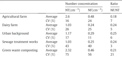
The number concentrations of the total andfluorescing particles (calculated using Eq. (1)), along with the number ratios offluorescent to total concentrations are listed inTable 4. The highest number concen-trations for total (NT = 2.6 cm−3) andfluorescent particles (NF = 0.48 cm−3) were recorded at the agricultural farm and green waste composting (NT = 2.32 cm−3, NF = 0.46 cm−3). In contrast, mean numberfluorescent fraction was lowest at the agricultural site (0.18) than other sites and less variable.

The coefficient of variation (the ratio of the standard deviation to the mean) revealed large variability in number concentration of both the total andfluorescent particles over the three measurements periods at Table 1

Summary details of sampling sites.

Site Description Sampling strategy

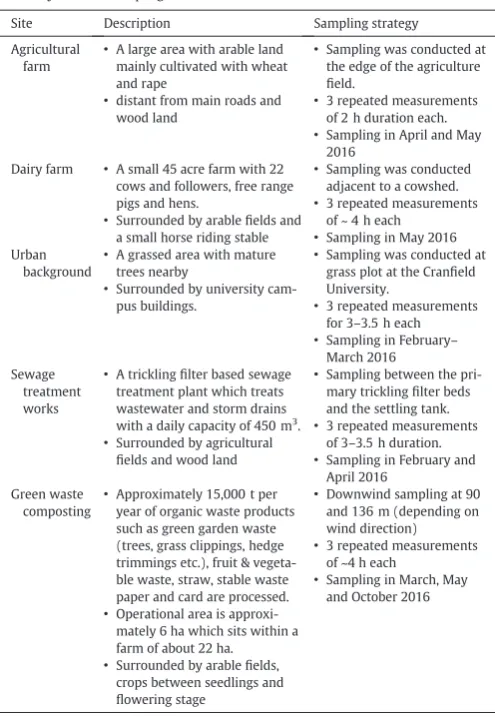
Agricultural farm

• A large area with arable land mainly cultivated with wheat and rape

• distant from main roads and wood land

• Sampling was conducted at the edge of the agriculture field.

• 3 repeated measurements of 2 h duration each. • Sampling in April and May

2016 Dairy farm • A small 45 acre farm with 22

cows and followers, free range pigs and hens.

• Surrounded by arablefields and a small horse riding stable

• Sampling was conducted adjacent to a cowshed. • 3 repeated measurements

of ~ 4 h each • Sampling in May 2016 Urban

background

• A grassed area with mature trees nearby

• Surrounded by university cam-pus buildings.

• Sampling was conducted at grass plot at the Cranfield University.

• 3 repeated measurements for 3–3.5 h each • Sampling in February–

March 2016 Sewage

treatment works

• A tricklingfilter based sewage treatment plant which treats wastewater and storm drains with a daily capacity of 450 m3

. • Surrounded by agricultural

fields and wood land

• Sampling between the pri-mary tricklingfilter beds and the settling tank. • 3 repeated measurements

of 3–3.5 h duration. • Sampling in February and

April 2016 Green waste

composting

• Approximately 15,000 t per year of organic waste products such as green garden waste (trees, grass clippings, hedge trimmings etc.), fruit & vegeta-ble waste, straw, stavegeta-ble waste paper and card are processed. • Operational area is

approxi-mately 6 ha which sits within a farm of about 22 ha. • Surrounded by arablefields,

crops between seedlings and flowering stage

• Downwind sampling at 90 and 136 m (depending on wind direction) • 3 repeated measurements

of ~4 h each

• Sampling in March, May and October 2016

Table 2

Fluorescence measurement channels (Ch) and wavelength ranges (nm).

Channel Lower wavelength Upper wavelength

1 298.2 316.4

2 316.4 344.8

3 344.9 362.5

4 377.5 401.5

5 401.5 429.7

6 430.2 457.5

7 456.7 485.6

8 486.0 514.0

9 514.1 542.0

10 542.0 569.8

11 569.9 597.6

12 597.6 625.2

13 625.3 652.8

14 652.8 680.2

15 680.3 707.5

the different sites, in particular at green waste composting and sewage treatment works (Table 3). This reflects significant impact of time-dependent site-specific factors on emissions, especially for industrial sources, and highlights the shortcomings of snapshot infrequent sam-pling to quantify magnitude and nature of bioaerosols emissions from environmental sources. Studies using the WIBS in different ambient en-vironments have reported similar variability in number concentrations of biological particles related to location and season.Gabey et al. (2010, 2011 and 2013)conducted studies in urban (winter), tropical and high altitude environments and observed bioaerosol number concentrations of 0.1 cm−3, 0.2–1.5 cm−3and 0.1 cm−3, respectively. Similarly, number concentrations offluorescent aerosol particles in an urban area reported byToprak and Schnaiter (2013)were variable across the seasons, being highest (0.046 cm−3) in summer and lowest in winter (0.019 cm−3). In the context of number concentrations of biological particles from industrial emissions, a recent study conducted using the WIBS at a green composting site showed a range of 0.10–0.30 cm−3during light and heavy workloads (O'Connor et al., 2015). By comparison, in our study, the average number concentration offluorescent particles at composting sites was 0.46 cm−3.

In terms of number weightedfluorescent fraction, the mean at different sites ranged from 0.18 (agricultural) to 0.25 (Urban background) with the highest variability across different measurements at the composting site (CV = 21%) again highlighting the impact of var-ious spatio-temporal factors on bioaerosol emissions. Atmospheric bioaerosols concentrations have been reported to be highly variable and can be affected by biological activity and meteorological factors (Toprak and Schnaiter, 2013;Bauer et al., 2008).Toprak and Schnaiter (2013)recently reported that number concentration fractions offl uo-rescent biological aerosol particles at an urban site during winter were from 0.0043–0.18. A similar study byO'Connor et al. (2015) at a composting site, with measurements using the WIBS, found that more than half of the total particles werefluorescent during heavy site activ-ity. In the present study,fluorescent particles represented up to 0.44 of total particles at ~ 100 m downwind of activity at the composting site. The observed differences are likely due to variability in microclimate, sampling characteristics and different size ranges (0.8–16 μm for Toprak and Schnaiter (2013)and 0.69 -∼13μm forO'Connor et al. (2015)). No direct comparison can be made between the present

investigation and these studies due to differences in the detectable range of particle size and specific environmental/sampling characteris-tics. Nonetheless, thesefindings show the impact of various sources/ac-tivities on temporal bioaerosols emissions loadings and the capability of real-time monitoring to identify sources and elucidate their level of con-tribution to atmospheric bioaerosols.

3.2. Fluorescence spectra from different environmental sources

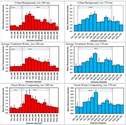
Fluorescence intensity across emission wavelength bands of the SIBS for the two excitation wavelengths (280 nm and 370 nm) for all the sites is illustrated inFigs. 1 and 2.

As afirst approach for qualitative description, emission spectra at each site are explained in terms of emission zones as a function of wavelength. The 280 nm excitationfluorescence spectra of the agri-cultural site shows peakfluorescence emission in 456.7–485.6 nm (Ch 7) and 569.9–597.6 nm (Ch 11) along with secondary peaks at 316.4–362.5 nm (Ch 2–3) and 625.3–652.8 nm (Ch 13) and 680_–707 nm (Ch15). In contrast, the 370 nm excitation_fluorescence spectrum had a sharp peak at 514–542 nm (Ch 9) with secondary peaks at 569.9–652.8 nm (Ch 11–13) and 680–734.7 nm (Ch 15_–16). At the dairy farm for both 280 nm and 370 nm excitation, the emission spectra were comparable to the agricultural site with slight differences at 569.9–652.8 nm (Ch 11–13) in secondary emis-sion modes.

The peak emission zone for 280 nm excitation, at urban background site, was centred at 456.7–485.6 nm (Ch 7) with secondary peaks at 316.4–344.8 nm (Ch 2), 542–569.85 (Ch 10), 597.6–625.2 nm (Ch 12) and 680.3–707.5 nm (Ch 15). Similarly, at 370 nm excitation, emission spectrum was multimodal with peaks at 514–542 nm (Ch 9), 597.6–625.2 nm (Ch 12) and 680.3–707.5 nm (Ch 15), respectively. The samples from sewage treatment works had a broad emission peak at 430.2–514 nm (Ch 6–8) followed by a secondary peak at 597.6–625.2 nm (Ch 12) and 680.3–707.5 nm (Ch 15), for 280 nm exci-tation. The emission spectrum for 370 nm excitation had peaks at 514–542 nm (Ch 9), 597.6–652.8 nm (Ch 12–13) and 680.3–707.5 nm (Ch 15).

For the green waste composting, the spectrum for 280 nm excitation was multimodal and characterised by afluorescence maximum at 430.2–485.6 nm (Ch 6–7) with secondary peaks at 316.4–344.8 nm (Ch 2), 486–542 nm (Ch 8–9) and 597.6–625.2 nm (Ch 12). In contrast, for the 370 nm excitation, the spectrum peaked at 514.1–542 (Ch 9) with shoulder peaks at 430.2–457.5 nm (Ch 6), 597.6–625.2 nm (Ch 12) and 680.3–734.7 nm (Ch 15–16).

In broader terms differences were found in the general shapes of the emissions spectra at different sites, in particular, the magnitude and wavelength of the secondary peaks at smaller and larger wavelengths than the maxima. Nevertheless, the assignment offluorescence to spe-cific biologicalfluorophores within atmospheric particles is challenging. Currently, a tangible explanation of the molecular origin offluorescence in different channels from particle population at these sites is unavail-able but based on existingfindings on LIF spectra of atmospherically rel-evant biologicalfluorophores assignments can be deduced. This can help to understand the underlying determinants of these differences and thus identifying distinctfluorescence signature of different environ-mental sources. The available literature on excitation and emission Table 3

Sample size of particles for the analysis offluorescence intensity across different wavelength bands at each site.

Sites Sampling 1

Number of particles

Sampling 2 Number of particles

Sampling 3 Number of particles

Total

Number of particles

Agricultural farm 16,329 12,611 20,213 49,153

Dairy farm 26,699 12,883 18,928 58,510

Urban background 25,830 19,744 28,035 73,609

Sewage treatment works 14,949 24,479 24,839 64,267

Green waste composting 24,412 15,046 4045 43,503

Table 4

Summary of particles concentrations at each site (number of measurementn= 3).

Number concentration Ratio

NT(cm−3) NF(cm−3) NF/NT

Agricultural farm Average 2.6 0.48 0.18

CV (%) 16 24 7

Dairy farm Average 1.03 0.24 0.24

CV (%) 26 25 5

Urban background Average 1.17 0.29 0.25

CV (%) 17 11 6

Sewage treatment works Average 1.03 0.25 0.24

CV (%) 43 40 3

Green waste composting Average 2.32 0.46 0.21

CV (%) 75 56 21

matrix spectra of a variety of biological_fluorophores can help to offer in-sights about the composition of particles (Hernandez et al., 2016; Pöhlker et al., 2012;Pan et al., 2010;Hill et al., 2009). According to the available data with respect to atmospherically relevant biological fluorophores, the emission wavelength from 400 to 500 nm is crowded by a number of biologicalfluorophores and emissions in this zone could originate from a mixed signal from a variety of compounds. In contrast, the emission zone from 500 to 700 is relatively clearer with compounds exhibiting largerΔλstokes (such as riboflavin, chlorophyllb). Whereas, emissions at 300–350 nm are characteristics of amino acids (Phenylala-nine, Tyrosine and Tryptophan).

Among thefive studied sites different emission zones atλex 280 nm could be assigned to amino acids (e.g. Tyrosine, tryptophan and phenyl-alanine in Ch 1_–3), several coenzymes/cofactors and structural biopoly-mers (e.g. pyridoxine, cellulose, neopterin, chitin, phenylocoumarin in Ch 4–8), andflavins in Ch 9–10. The potential source of emission in Ch 4–10 (377.5–569.8 nm) forλex 370 could be from diverse coen-zymes/cofactors (NADPH,flavins, neopterin, lumazine) and a range of structural biopolymer or their constituents (cellulose, chitin, ferulic acids, phenylocoumarin). The emission in Ch 11–16 (569.9–734.7 nm) could be from secondary metabolites (e.g. Alkaloids, terpenoids) and pigments (e.g. Chlorophyll). However, secondary metabolites and age-related pigments have been reported to have broad emission bands and could contribute in Ch 5–Ch 16 for bothλex 280 andλex 370. For example, forλex 250–395 nm, terpenoids from plants and fungi have reportedλem in the range of 400–725 nm and lipofuscin hasλem in the range of 430–670 nm for λex 260–280 nm and 340–490 nm (Pöhlker et al., 2012).

The primary peaks, for both 280 nm and 370 nm excitation, at differ-ent sites was at 430–514 nm (Ch 6–8) and 514.1–542 (Ch 9), respec-tively. The predominant emission in Ch 6–8 (430–514 nm) is possibly from structural compounds (cellulose (dry), chitin (Dry), lignin (phenylcoumarin), and coenzyme (e.g. Neopterin). While the emission at 514.1–542 (Ch 9) for 370 nm excitation can be assigned toflavins. The secondary peaks for both the excitation wavelengths are centred

in Ch 11 (596.9_–597.6 nm), Ch 12 (597.6_–625.2 nm), Ch 13 (625.3–652.8 nm), and Ch 15–16 (680.3–734.7 nm) of the spectra and relevant biologicalfluorophore in this region are likely to be from sec-ondary metabolites (e.g. alkaloids, terpenoids) pigments (e.g. chloro-phyll,flavonoids, lipofuscin). Lipofuscins are age-related pigments reported to be formed due to oxidative stress and has a wide emission range from blue to red (Roshchina, 2012), whereas emissions in Ch 1–3 (298–362 nm) are reported to be from amino acids. The differ-ences in secondary emission peaks at different sites suggest that compounds with weakfluorescence could play a role in selectivity. Al-though the emission wavelengths with the highest intensity constitute the dominant mode of the spectra the contribution from low emission intensity at a specific wavelength is of value to disentangle the mixed fluorescence singles from a source. This assessment could inform the development of hypotheses on how and why molecular composition varies between particle populations at different sites which can be tested in further experimentations and analysis.

The secondary emission peaks for bothλex 280 andλex 370 were variable across sites and centered at lower and larger wavelength than maxima. The observed shift in emission modes at smaller and larger wavelengths than the peaks at different sites could be due to the under-lying differences in chemical composition of emissions at these sites. However, in the natural environment, bioaerosols are part of a complex mixture differing significantly from lab-based studies. This diversity of biological and non-biological interfering compounds significantly hampers the selectivity of LIF based bioaerosol detectors. Therefore, assigning a spectral response to the classification of bioaerosols is the big-gest challenge due to wide emission bands and overlappingfluorescence signatures. The SIBS tackles this challenge with an improved spectral res-olution to elucidate spectrally integrated signals by measuringfl uores-cence emission spectra in 16 wavelength bands. In the case of the WIBS the three emission bands FL1 (λex = 280 nm,λem∼310–400 nm), FL2 (λex = 280 nm,λem∼420–650 nm) and FL3 (λex = 370 nm,λem ∼420–650 nm) will give an integrated signals for a range offluorophores. Proteins and coenzymes are likely to dominate the emission signal in FL1

Agricultural Farm_λex 280 nm

Agricultural_λex 370 nm

Dairy Farm_λex 280 nm

Dairy Farm_λex 370 nm

and structural compounds along with certain coenzymes are likely to be detected in FL2. Similarly, the emission spectral region for FL3 can only detect an integratedfluorescence for a range of coenzymes, structural compounds and secondary metabolites. Therefore, offering poor selectiv-ity for a specific biologicalfluorophore and hence limiting the suitability of these emission bands to discriminate bioaerosols. For instance, the as-sumption about FL3 emissions as an indicator of metabolic state may not hold true due to the diversity of biologicalfluorophore emitting in this range. Furthermore, WIBS is unlikely to detect compounds with largerΔλstokes (chlorophyll or secondary metabolites). In contrast, it can be seen that highly resolvedfluorescence intensity measure-ments by the SIBS provides more detailed spectral information as compared to broad emission bands in the WIBS and that the addi-tional channels in the SIBS are revealing information that is lost in the WIBS (Figs. 1 and 2). However extensive laboratory studies are yet to be performed to offer meaningful interpretations of this addi-tional spectral information in the context of complex ambient aero-sol samples. Hence, the above description is an overview of the capability of improved spectral resolution to elucidate spectrally in-tegrated signals from contrasting environmental sources based on lab-based measurements on excitation and emission matrix spectra of the most relevant biologicalfluorophores.

In terms of particle size of the sample data for_fluorescence spectra analysis inFigs. 1 and 2, most of the particles measured at these sites were predominantly offine size fraction. The mean particle size ranged from 0.59μm (Sewage treatment works) to 0.87μm (Green waste composting) with considerable variation at each site (Table 5).

Thefluorescence in these size fractions (below 1μm) could orig-inate from the contribution from cellular fragments or molecular de-composition products of biological material as well as non-biological materials. Further studies are required to address the molecular ori-gin offluorescence infine and ultrafine particles in the air and to es-tablish their relevance and implications to characterise bioaerosols

Urban Background_λex 280 nm

Urban Background_λex 370 nm

Sewage Treatment Works_λex 280 nm

Sewage Treatment Works_λex 370 nm

Green Waste Composting_λex 280 nm

Green Waste Composting_λex 370 nm

Fig. 2.Meanfluorescence spectra for two excitation wavelengths at the urban background, sewage treatment works and green waste composting. Bars = standard deviation. (For interpretation of the references to colour in thisfigure legend, the reader is referred to the web version of this article.)

Table 5

Particle size (μm) of sample data forfluorescence spectra analysis at different sites (n = number of particles).

Site Mean Minimum Maximum Standard deviation

emissions. Fluorescence properties of afluorophore are highly de-pendent on the molecular environment and this in biological cells or their fragments could be much more dynamic and complex lead-ing to differences in intensity and emission modes in atmospheric bioaerosols in comparison to lab-based studies of pure biological fluorophores (Pan, 2015). Furthermore, atmospheric aerosols from both anthropogenic and natural sources have a range of biological and non-biologicalfluorescent constituents and therefore emission spectra are characterised by mixed signals from differentfluorophores. Non-biological compounds such as secondary organic aerosols, mineral dust and polycyclic aromatic hydrocarbons can cause positivefl uores-cence measurement artefacts. Consequently, a selective assignment of the molecular origin offluorescence is not straightforward. Thus differ-ences in emission intensity should be viewed as semi-quantitative and analysed adjunct to overall spectra.

4. Conclusions and future directions

The capability and utility of a novel LIF sensor based on dual-wavelength excitation with highly resolvedfluorescence intensity mea-surements (Spectral Intensity Bioaerosol Sensor (SIBS)) to characterise bioaerosols emissions in real time was evaluated. The number concen-tration of total andfluorescent particles was highly variable across the sites. Emission spectra from different sites were multimodal with inten-sity differences at some channels for both excitation wavelengths. It has been demonstrated that highly resolved emission intensity measure-ments by the SIBS provides additional spectral information in compari-son to the WIBS. This demonstrates that SIBS can contribute to overcoming the selectivity challenges to discriminate and classify bioaerosols emissions. However, improved numerical methods and tools are needed to utilise this detailed information to develop discrim-ination algorithms. Different post detection methods (e.g. principal component analysis, Hierarchical agglomerative cluster analysis, Linear discriminant analysis) have been proposed and used to discriminate bi-ological classes and other interferants (Crawford et al., 2015;Pan, 2015; Robinson et al., 2013;Pan et al., 2010) with data from existing LIF based instruments. These approaches and methodologies are evolving and deemed suitable for SIBS data but are yet to be tested to develop an optimised classification method. However, there is pressing need to conduct lab-based studies with atmospherically relevant biological fluorophores/aerosols in order to build comprehensive SIBSfl uores-cence spectra library. Such library will greatly contribute to the elucida-tion of spectrally integrated signals and thus improving measurement selectivity for bioaerosols emissions. At the same time, comparative measurements of SIBS with other biochemical detection methods focus-ing on various constituents (endotoxin, peptidoglycans,β1–3 glucan, DNA) or metabolites (mVOC) (qPCR, LAL, GC–MS,flow cytometry) and development of improved analysis methods to analyse the complex set of data generated by the SIBS will advance the use of single particle LIF based technique as a powerful analytical tool to characterise bioaerosols emissions from environmental sources.

5. Limitations of the study

The SIBS is a beta version device and the measurements reported in this paper were one of the earliest versions of the SIBS with limited data analysis capability. One of the limitations of this study, for example, is that we used a singlefluorescence threshold value to calculate number concentration offluorescent particles. Ideally, individual lowerfl uores-cence threshold limits for all the channels should be set to derive wave-length basedfluorescent particle time series data (channel by channel). Thefluorescence spectra analysis, however, is carried out by subtracting mean forced trigger emission intensity values from the particle by par-ticle emission intensity values in corresponding channels. Nonetheless, the results should be interpreted with caution.

Acknowledgments

This work was supported by the Natural Environment Research Council [NE/M01163/1]. This award is made under the auspices of the Environmental Microbiology and Human Health programme. This work represents the views of the results and the research and not the views of the funders. The comments from Darrel Baumgardner (Droplet Mea-surement Technologies) are gratefully acknowledged. The data will be available on 1ST July 2020 via the Environmental Information Data Cen-tre, the Natural Environment Research Council's long-term data reposi-tory for terrestrial and freshwater scienceshttps://catalogue.ceh.ac.uk/ eidc/documents.

Appendix A. Supplementary data

Supplementary data to this article can be found online athttps://doi. org/10.1016/j.scitotenv.2018.08.120.

References

Anderson, B.D., Ma, M., Xia, Y., Wang, T., Shu, B., Lednicky, J.A., Ma, M.J., Lu, J., Gray, G.C., 2016.Bioaerosol sampling in modern agriculture: a novel approach for emerging pathogen surveillance? J. Infect. Dis. 214 (4), 537–545.

Bauer, H., Schueller, E., Weinke, G., Berger, A., Hitzenberger, R., Marr, I.L., Puxbaum, H., 2008.Significant contributions of fungal spores to the organic carbon and to the aero-sol mass balance of the urban atmospheric aeroaero-sol. Atmos. Environ. 42 (22), 5542–5549.

Borlée, F., Yzermans, C.J., van Dijk, C.E., Heederik, D., Smit, L.A., 2015.Increased respiratory symptoms in COPD patients living in the vicinity of livestock farms. Eur. Respir. J. 46 (6), 1605–1614.

Bünger, J., Schappler-Scheele, B., Hilgers, R., Hallier, E., 2007.A 5-year follow-up study on respiratory disorders and lung function in workers exposed to organic dust from composting plants. Int. Arch. Occup. Environ. Health 80 (4), 306–312.

Crawford, I., Ruske, S., Topping, D.O., Gallagher, M.W., 2015.Evaluation of hierarchical ag-glomerative cluster analysis methods for discrimination of primary biological aerosol. Atmos. Meas. Tech. 8 (11), 4979.

Crawford, I., Lloyd, G., Herrmann, E., Hoyle, C.R., Bower, K.N., Connolly, P.J., Flynn, M.J., Kaye, P.H., Choularton, T.W., Gallagher, M.W., 2016.Observations offluorescent aerosol–cloud interactions in the free troposphere at the High-Altitude Research Sta-tion Jungfraujoch. Atmos. Chem. Phys. 16 (4), 2273–2284.

van der Hoek, W., Morroy, G., Renders, N.H., Wever, P.C., Hermans, M.H., Leenders, A.C., Schneeberger, P.M., 2012.Epidemic Q fever in humans in the Netherlands. Adv. Exp. Med. Biol. 984, 329–364.

Douglas, P., Bakolis, I., Fecht, D., Pearson, C., Sanchez, M.L., Kinnersley, R., de Hoogh, K., Hansell, A.L., 2016.Respiratory hospital admission risk near large composting facili-ties. Int. J. Hyg. Environ. Health 219 (4–5), 372–379.

Gabey, A.M., Gallagher, M.W., Whitehead, J., Dorsey, J.R., Kaye, P.H., Stanley, W.R., 2010. Measurements and comparison of primary biological aerosol above and below a trop-ical forest canopy using a dual channelfluorescence spectrometer. Atmos. Chem. Phys. 10 (10), 4453–4466.

Gabey, A.M., Stanley, W.R., Gallagher, M.W., Kaye, P.H., 2011.Thefluorescence properties of aerosol larger than 0.8μm in urban and tropical rainforest locations. Atmos. Chem. Phys. 11 (11), 5491–5504.

Gabey, A.M., Vaitilingom, M., Freney, E., Boulon, J., Sellegri, K., Gallagher, M.W., Crawford, I.P., Robinson, N.H., Stanley, W.R., Kaye, P.H., 2013.Observations offluorescent and bi-ological aerosol at a high-altitude site in central France. Atmos. Chem. Phys. 13 (15), 7415–7428.

Hallar, A., Chirokova, G., McCubbin, I., Painter, T.H., Wiedinmyer, C., Dodson, C., 2011. At-mospheric bioaerosols transported via dust storms in the western United States. Geophys. Res. Lett. 38 (17).

Hernandez, M., Perring, A.E., McCabe, K., Kok, G., Granger, G., Baumgardner, D., 2016. Chamber catalogues of optical andfluorescent signatures distinguish bioaerosol clas-ses. Atmos. Meas. Tech. 9 (7), 3283–3292.

Hill, S.C., Mayo, M.W., Chang, R.K., 2009.Fluorescence of Bacteria, Pollens, and Naturally Occurring Airborne Particles: Excitation/Emission Spectra (No. ARL-TR-4722). U.S. Army Research Lab, Adelphi.

Huffman, J.A., Treutlein, B., Pöschl, U., 2010.Fluorescent biological aerosol particle concen-trations and size distributions measured with an ultraviolet aerodynamic particle sizer (UV-APS) in Central Europe. Atmos. Chem. Phys. 10 (7), 3215–3233. Huffman, J.A., Sinha, B., Garland, R.M., Snee-Pollmann, A., Gunthe, S.S., Artaxo, P., Martin,

S.T., Andreae, M.O., Pöschl, U., 2012.Size distributions and temporal variations of bi-ological aerosol particles in the Amazon rainforest characterized by microscopy and real-time UV-APSfluorescence techniques during AMAZE-08. Atmos. Chem. Phys. 12 (24), 11997–12019.

Huffman, A., Prenni, J., DeMott, J., Pohlker, C., Mason, H., Robinson, H., Frohlich-Nowoisky, J., Tobo, Y., Despres, R., Garcia, E., Gochis, J., 2013.High concentrations of biological aerosol particles and ice nuclei during and after rain. Atmos. Chem. Phys. 13 (13), 6151–6164. Jahne, M.A., Rogers, S.W., Holsen, T.M., Grimberg, S.J., Ramler, I.P., Kim, S., 2016.Bioaerosol

Kaye, P.H., Stanley, W.R., Hirst, E., Foot, E.V., Baxter, K.L., Barrington, S.J., 2005.Single par-ticle multichannel bio-aerosolfluorescence sensor. Opt. Express 13 (10), 3583–3593. Li, J., Zhou, L., Zhang, X., Xu, C., Dong, L., Yao, M., 2016.Bioaerosol emissions and detection of airborne antibiotic resistance genes from a wastewater treatment plant. Atmos. Environ. 124, 404–412.

Madsen, A.M., Thilsing, T., Bælum, J., Garde, A.H., Vogel, U., 2016.Occupational exposure levels of bioaerosol components are associated with serum levels of the acute phase protein Serum Amyloid A in greenhouse workers. Environ. Health 15 (1), 9. Mazar, Y., Cytryn, E., Erel, Y., Rudich, Y., 2016.Effect of dust storms on the atmospheric

microbiome in the Eastern Mediterranean. Environ. Sci. Technol. 50 (8), 4194–4202. Morris, C.E., Leyronas, C., Nicot, P.C., 2014.Movement of bioaerosols in the atmosphere and the consequences for climate and microbial evolution. In: Colbeck, I., Lazaridis, M. (Eds.), Aerosol Science: Technology and Applications. John Wiley & Sons Ltd., pp. 393–415.

O'Connor, A.M., Auvermann, B., Bickett-Weddle, D., Kirkhorn, S., Sargeant, J.M., Ramirez, A., Von Essen, S.G., 2010.The association between proximity to animal feeding oper-ations and community health: a systematic review. PLoS ONE 5 (3), e9530. O'Connor, D.J., Healy, D.A., Hellebust, S., Buters, J.T., Sodeau, J.R., 2014.Using the WIBS-4

(Waveband Integrated Bioaerosol Sensor) technique for the on-line detection of pol-len grains. Aerosol Sci. Technol. 48 (4), 341–349.

O'Connor, D.J., Daly, S.M., Sodeau, J.R., 2015.On-line monitoring of airborne bioaerosols released from a composting/green waste site. Waste Manag. 42, 23–30.

Pan, Y.L., 2015.Detection and characterization of biological and other organic-carbon aerosol particles in atmosphere usingfluorescence. J. Quant. Spectrosc. Radiat. Transf. 150, 12–35.

Pan, Y.L., Hill, S.C., Pinnick, R.G., Huang, H., Bottiger, J.R., Chang, R.K., 2010.Fluorescence spectra of atmospheric aerosol particles measured using one or two excitation wave-lengths: comparison of classification schemes employing different emission and scat-tering results. Opt. Express 18 (12), 12436–12457.

Pankhurst, L.J., Whitby, C., Pawlett, M., Larcombe, L.D., McKew, B., Deacon, L.J., Morgan, S.L., Villa, R., Drew, G.H., Tyrrel, S., Pollard, S.J., 2012.Temporal and spatial changes in the microbial bioaerosol communities in green-waste composting. FEMS Microbiol. Ecol. 79 (1), 229–239.

Pearce, D.A., Alekhina, I.A., Terauds, A., Wilmotte, A., Quesada, A., Edwards, A., Dommergue, A., Sattler, B., Adams, B.J., Magalhães, C., Chu, W.L., 2016.Aerobiology over Antarctica–a new initiative for atmospheric ecology. Front. Microbiol. 7, 16. Pearson, C., Littlewood, E., Douglas, P., Robertson, S., Gant, T.W., Hansell, A.L., 2015.

Expo-sures and health outcomes in relation to bioaerosol emissions from composting facil-ities: a systematic review of occupational and community studies. J. Toxicol. Environ. Health B 18 (1), 43–69.

Perring, A.E., Schwarz, J.P., Baumgardner, D., Hernandez, M.T., Spracklen, D.V., Heald, C.L., Gao, R.S., Kok, G., McMeeking, G.R., McQuaid, J.B., Fahey, D.W., 2015.Airborne obser-vations of regional variation influorescent aerosol across the United States. J. Geophys. Res. Atmos. 120 (3), 1153–1170.

Pöhlker, C., Huffman, J.A., Pöschl, U., 2012.Autofluorescence of atmospheric bioaerosols– fluorescent biomolecules and potential interferences. Atmos. Meas. Tech. 5 (1), 37–71.

Robinson, N.H., Allan, J.D., Huffman, J.A., Kaye, P.H., Foot, V.E., Gallagher, M., 2013.Cluster analysis of WIBS single-particle bioaerosol data. Atmos. Meas. Tech. 6 (2), 337. Roshchina, V.V., 2012. Vital autofluorescence: application to the study of plant living cells.

Int. J. Spectrosc., 124672https://doi.org/10.1155/2012/124672(14 pages).

Saari, S., Niemi, J., Rönkkö, T., Kuuluvainen, H., Järvinen, A., Pirjola, L., Aurela, M., Hillamo, R., Keskinen, J., 2015.Seasonal and diurnal variations offluorescent bioaerosol con-centration and size distribution in the urban environment. Aerosol Air Qual. Res. 15 (2), 572–581.

Schumacher, C.J., Pöhlker, C., Aalto, P., Hiltunen, V., Petäjä, T., Kulmala, M., Pöschl, U., Huffman, J.A., 2013.Seasonal cycles offluorescent biological aerosol particles in bo-real and semi-arid forests of Finland and Colorado. Atmos. Chem. Phys. 13 (23), 11987–12001.

Sialve, B., Gales, A., Hamelin, J., Wery, N., Steyer, J.P., 2015.Bioaerosol emissions from open microalgal processes and their potential environmental impacts: what can be learned from natural and anthropogenic aquatic environments? Curr. Opin. Biotechnol. 33, 279–286.

Sun, J., Ariya, P.A., 2006.Atmospheric organic and bio-aerosols as cloud condensation nu-clei (CCN): a review. Atmos. Environ. 40 (5), 795–820.

Sykes, P., Jones, K., Wildsmith, J.D., 2007.Managing the potential public health risks from bioaerosol liberation at commercial composting sites in the UK: an analysis of the ev-idence base. Resour. Conserv. Recycl. 52 (2), 410–424.

Taha, M.P.M., Pollard, S.J., Sarkar, U., Longhurst, P., 2005.Estimating fugitive bioaerosol re-leases from static compost windrows: feasibility of a portable wind tunnel approach. Waste Manag. 25 (4), 445–450.

Taha, M.P.M., Drew, G.H., Longhurst, P.J., Smith, R., Pollard, S.J., 2006.Bioaerosol releases from compost facilities: evaluating passive and active source terms at a green waste facility for improved risk assessments. Atmos. Environ. 40 (6), 1159–1169. Taha, M.P.M., Drew, G.H., Vestlund, A.T., Aldred, D., Longhurst, P.J., Pollard, S.J., 2007.

Enu-merating actinomycetes in compost bioaerosols at source—use of soil compost agar to address plate‘masking’. Atmos. Environ. 41 (22), 4759–4765.

Toprak, E., Schnaiter, M., 2013.Fluorescent biological aerosol particles measured with the Waveband Integrated Bioaerosol Sensor WIBS-4: laboratory tests combined with a one yearfield study. Atmos. Chem. Phys. 13 (1), 225–243.

Vestlund, A.T., Al-Ashaab, R., Tyrrel, S.F., Longhurst, P.J., Pollard, S.J., Drew, G.H., 2014. Mor-phological classification of bioaerosols from composting using scanning electron mi-croscopy. Waste Manag. 34 (7), 1101–1108.

Walser, S.M., Gerstner, D.G., Brenner, B., Bünger, J., Eikmann, T., Janssen, B., Kolb, S., Kolk, A., Nowak, D., Raulf, M., Sagunski, H., 2015.Evaluation of exposure–response relation-ships for health effects of microbial bioaerosols–a systematic review. Int. J. Hyg. Envi-ron. Health 218 (7), 577–589.

Wei, K., Zou, Z., Zheng, Y., Li, J., Shen, F., Wu, C.Y., Yao, M., 2016.Ambient bioaerosol par-ticle dynamics observed during haze and sunny days in Beijing. Sci. Total Environ. 550, 751–759.

Yu, X., Wang, Z., Zhang, M., Kuhn, U., Xie, Z., Cheng, Y., Pöschl, U., Su, H., 2016.Ambient measurement offluorescent aerosol particles with a WIBS in the Yangtze River Delta of China: potential impacts of combustion-related aerosol particles. Atmos. Chem. Phys. 16 (17), 11337–11348.