Flow Separation Control over a Rounded Ramp with Spanwise Alternating
Wall Actuation
Weidan Ni (
倪玮丹
)
1,2, Lipeng Lu (
陆利蓬
)
1,3, Jian Fang (
方剑
)
2, Charles
Moulinec
2, David R Emerson
2and Yufeng Yao (姚宇峰)
41National Key Laboratory of Science and Technology on Aero-Engine Aero-Thermodynamics, School of
Energy and Power Engineering, Beihang University, Beijing, 100191, China
2Scientific Computing Department, Science & Technology Facilities Council (STFC), Daresbury
Laboratory, Warrington, WA4 4AD, UK
3 Collaborative Innovation Center of Advanced Aero-Engine, Beijing 100191, China
4Faculty of Environment and Technology, Department of Engineering Design and Mathematics, University
of the West of England, Bristol, BS16 1QY, UK
Abstract An implicit large-eddy simulation is carried out to study turbulent boundary-layer separation from a backward-facing
rounded ramp with active wall actuation control. This method, called spanwise alternating distributed strips control, is imposed
onto the flat plate surface upstream of a rounded ramp by alternatively applying out-of-phase control and in-phase control to
the wall-normal velocity component in the spanwise direction. As a result, the local turbulence intensity is alternatively
suppressed and enhanced, leading to the creation of vertical shear-layers, which is responsible for the presence of large-scale
streamwise vortices. These vortices exert a predominant influence on the suppression of the flow separation. The interaction
between the large-scale vortices and the downstream recirculation zone and free shear-layer is studied by examining flow
statistics. It is found that in comparison with the non-controlled case the flow separation is delayed, the reattachment point is
shifted upstream, and the length of the mean recirculation zone is reduced up to 8.49%. The optimal control case is achieved
with narrow in-phase control strips. An in-depth analysis shows that the delay of the flow separation is attributed to the
activation of the near-wall turbulence by the in-phase control strips and the improvement of the reattachment location is mainly
due to the large-scale streamwise vortices, which enhance the momentum transport between the main flow and separated region.
Keywords Implicit Large-eddy Simulation (ILES), Backward-Facing Rounded Ramp, Spanwise Alternating Distributed Strips
(SADS) Control, Turbulent Secondary Flow, Flow Separation and Reattachment
I. INTRODUCTION
Flow control can involve passive or active devices that are able to induce favourable flow characteristics. As noted by
Gad-el-Hak [1], modern flow control was introduced by Prandtl [2] using boundary-layer theory with a discussion of
experiments where the boundary layer was controlled. Historically, it is clear that boundary-layer control is one of the oldest
and most critical aspects of existing flow control methods [3]. In general, flow separation is considered to have negative effects,
including an increase in pressure drag, flow blockage, loss of lift, instability, and stall and surge phenomena. Leschziner et al.
2
suppression of separation, in which the latter aims to reduce the pressure drag by suppressing flow separation mainly via
momentum transport enhancement. Passive vortex generators (VGs), comprised of arrays of ribs and grooves aligned in the
streamwise direction with the order of the local boundary-layer thickness, have been used to control flow separation since
Taylor [5] first introduced this control strategy in the late 1940s. The generated large-scale streamwise vortices (LSSVs) by
VGs, which can enhance the momentum transport in the boundary layer, are believed to be crucial. Lin [6] showed that
low-profile VGs, defined as those with a device height between 10% and 50% of the boundary-layer thickness, can produce
streamwise vortices just strong enough to overcome separation without unnecessarily persisting within the boundary layer once
the flow control objective is achieved. While this concept works well, VGs still face certain technical difficulties in practical
applications such as design integration and manufacturing because of local shape change.
In addition to vortex generators, it has been found that some small-scale passive control strategies, such as alternatively
distributed riblets or wall roughness imposed within a turbulent boundary layer, could also induce LSSVs. The first evidence
appeared in 2002 when Koeltzsch et al. [7] applied convergent and divergent riblets to the inside wall of a turbulent pipe-flow.
This study primarily focused on providing a hydrodynamic explanation for the converging texture found on the skin
surrounding the sensory receptors of fast swimming sharks. Through tiny surface modifications at the pipe wall, a herringbone
riblet arrangement was able to impose large-scale modes onto the outer region of the pipe flow. Nugroho et al. [8] extended
this research and found that large-scale spanwise periodicity could be induced in a boundary layer by applying a
converging-diverging riblet-type surface roughness in a zero-pressure-gradient turbulent boundary layer. Further analysis of the
pre-multiplied energy spectra suggested surface roughness radically modifies the largest scale energetic structures. The
characteristics of a turbulent boundary layer overlying a complex roughness topography were experimentally explored by
Mejia-Alvarez et al. [9,10]. A lateral exchange of low- and high-momentum pathways (LMP/HMP, respectively) was observed.
Mejia-Alvarez et al. [10] suggested that the large-scale LMP/HMP are different from the instantaneous low- and
high-momentum regions [11-15]. They could further provide preferential pathways for the instantaneous large-scale motions. The
same topography was then studied by Barros et al. [16] using stereo particle image velocimetry measurements in the
wall-normal-spanwise plane. The spanwise regions between LMPs and HMPs are occupied by swirling motions, suggesting the
generation and sustainment of turbulent secondary flows due to the spanwise heterogeneity of the complex roughness under
consideration. Turbulent wall-bounded flows over transverse roughness transitions were studied by Willingham et al. [17] by
using large-eddy simulation (LES). The results showed that LMPs are spatially stationary and flanked by 𝛿-scale (local
turbulent boundary-layer thickness) counter-rotating vortices which serve to pump fluid vertically from the wall, ultimately
3
[18] carried out an experimental investigation on the modifications of turbulence over a wall with spanwise-varying roughness
using particle image velocimetry and hotwire anemometry. Conditional average analyses revealed that the observed
time-invariant flow structures result from the time-averaged process of instantaneous turbulent events that occur frequently in some
scenario. Kevin et al. [19] also suggested that the mean secondary flows arise from the averaged process of relatively strong
turbulent events that occur preferentially in both time and space. Hinze et al. [20,21] analysed secondary motions based on
turbulent production and dissipation by applying the usual boundary-layer approximations to the balance equations for
turbulence kinetic energy (TKE). They suggested that when the production is greater than the dissipation in a localised region,
the poor fluid is transported into this region by the generated secondary flow, and in the meantime, the
turbulence-rich fluid is flowing out of the region and vice versa.
Parametric investigations of the characteristics of large-scale vortices induced by spanwise inhomogeneity have also been
carried out. Nugroho et al. [8] suggested that increasing the converging-diverging angle or the viscous-scaled height of riblets
resulted in stronger spanwise perturbations. Increasing the fetch seems to cause the perturbations to grow further from the
surface, while the overall strength of the induced low- and high-speed regions remains relatively unaltered. Willingham et al.
[17] found varying the width of the high-roughness strips (𝐿𝑠) had a strong impact on the secondary flow pattern whereas the
variations in the ratio of the high roughness length to the low roughness length (λ) imposed a mild effect. The effect of the strip
width on the secondary flow topology was investigated by Stroh et al. [22], based on results from a turbulent channel flow with
spanwise alternating distributed no-slip and free-slip regions. Using direct numerical simulation (DNS), they found that the
width of the free-slip area (note that the effect of free-slip area on the flow field is similar with the low-roughness regions for
the flows over rough walls) might be a relevant scaling parameter for the secondary flow topology while the influence of the
no-slip spacing is weaker, which is opposite to the conclusion drawn by Willingham et al. [17]. Recently, Hwang et al. [23]
systematically studied the two parameters of the pitch (P) and width (S) for roughness elements in turbulent boundary layer
over longitudinal surface roughness using DNS. Their analysis showed that the size of the secondary flow is mostly determined
by the value of P−S, i.e., the valley width. This is consistent with the results obtained by Stroh et al. [22] that the width of the
free-slip region in wall units appears to be an important parameter for the vortex formation. Vanderwel et al. [24] concluded
that the large-scale secondary flows are accentuated when the adjacent spacing of the roughness elements is roughly
proportional to the boundary-layer thickness. Cases with coarser spacings also generate 𝛿-scale secondary flows with tertiary
flows located at the centres of the valleys between the elevated roughness strips. Yang et al. [25] assessed how the spacing
between the adjacent high roughness rows, sy, affects the turbulence structure in channel flows at high Reynolds number. The
4
in a turbulent channel flow controlled by alternately imposed patches of high and low wall shear stress in the lateral direction
on the lower wall of the channel. The effect of the lateral spacing, s, of the uniform-stress patches (for both high and low wall
shear stress) on the similarity and structure of turbulent inertial motion was investigated. They found that the global outer-layer
similarity is maintained when s is less than around 0.39H or greater than about 6.28H, where H is the half-height of the channel.
The effect of the Reynolds number on the flow field was also studied by Stroh et al. [22]. They suggested that flows at 𝑅𝑒𝜏 =
120 and 360 reveal a very similar flow topology transition to the one at 𝑅𝑒𝜏 = 180 with the spanwise wavelength of the no-slip
and free-slip strips increasing, implying Reynolds number independence of the proposed control method in a turbulent channel
flow.
Mejia-Alvarez et al. [9,10], Willingham et al. [17] and Anderson et al. [27] suggested that the transverse variation of the
surface drag induced a vertical shear-layer, which caused the spanwise transfer of low- and high-momentum fluids and then
led to the generation of a 𝛿-scale secondary flow. Willingham et al. [17] stated that the LMP constitutes Prandtl’s second kind
of secondary flow. Anderson et al. [27] confirmed that this mean secondary flow is Prandtl’s second kind of secondary flow,
both driven and sustained by spatial gradients in the Reynolds-stress components, which cause a subsequent imbalance between
production and dissipation of turbulent kinetic energy that necessitates secondary advective velocities. As Townsend [28]
proposed, the large-scale secondary motions generated as previously mentioned could be sustained due to the transverse
gradients of the imposed stress on the bounding surface. Recently, Xu et al. [29] investigated the development of a laminar
boundary layer over a rectangular convergent-divergent riblet section in a water flume. They found that the fluid inside the
riblet valley follows a helicoidal path and interacts with the crossflow playing an important role in determining the structure of
the secondary flow. As Vanderwel et al. [24] anticipated, because these secondary flows have such a large impact on the
structure of the boundary layer, and can be created easily by modifying the surface topology, these flows could have important
consequences for near-wall mixing, drag reduction, and flow control. Therefore, it is informative to further investigate the
characteristics of LSSVs generated by these control devices and the underlying mechanisms, as well as their effectiveness in
suppressing boundary-layer separation.
Many experiments and numerical simulations have been devoted to spanwise heterogeneity control, but most of the
research is limited to simple geometries, such as a flat plate boundary layer [8-10,16,17,24,26,30,31] or planar channel flow
[22,25,29,32-34]. The study of spanwise-heterogeneity small-scale control in separated flows has never been reported to the
authors’ knowledge. In this paper, spanwise alternating distributed strips (SADS), composed of alternatively imposed
backward-5
facing rounded ramp. The control method was developed by Ni et al. [33,34] and they showed that LSSVs, whose scale can be
up to the half-height of channel, could be generated by small-scale wall actuation. This paper aims to investigate SADS control
in separated flow to assess the performance of this control strategy in suppressing flow separation, focusing on the fundamental
mechanisms of the flow control. The active wall actuation, which is difficult to be implemented in practical application, is
taken as an effective approach to realise the spanwise heterogeneities. The computational geometry under consideration is a
turbulent flow over a backward-facing rounded ramp, which has been studied by Lardeau et al. [35] and Bentaleb et al. [36].
The simulations are carried out using implicit large-eddy simulation (ILES) at a Reynolds number of Re = 7,106 (based on the
freestream velocity and the height of the rounded ramp H) and at a low Mach number of M = 0.2. A relatively low Reynolds
number is considered to avoid the interactions between the outer-layer large-scale structures of a natural turbulent boundary
layer as observed by Hutchins and Marusic [37] and the possible large-scale motions induced by SADS control. Four controlled
cases with different widths of IPC/OPC strips are simulated in the present study to investigate the effect of the strip width,
among which two cases are analysed in detail and optimised controlling parameters are finally suggested.
II. METHODOLOGIES
The governing equations are described first, followed by an introduction of the numerical method and computational setup.
A. Governing Equations
The three-dimensional (3-D) unsteady compressible Navier-Stokes (N-S) equations in a general, time-invariant system are
solved numerically in a strong conservation non-dimensional form as,
𝜕𝑸 𝜕𝑡 +
𝜕𝑬𝑖 𝜕𝑥𝑖 =
𝜕𝑭𝑖
𝜕𝑥𝑖 (1)
In Eq. (1), 𝑸 = [𝜌, 𝜌𝑢, 𝜌𝑣, 𝜌𝑤, 𝜌𝑒]T is the solution vector. The primary variables are the density 𝜌, the velocity
components u, v and w and the total energy per unit mass e. The static temperature T and pressure P are related to the density
𝜌 via the equation of state of an ideal gas, 𝑃 = 𝜌𝑇
𝛾𝑀2. All the variables in the N-S equations are normalised by the reference
parameters except additional descriptions. The N-S equations are non-dimensionalised with the reference density 𝜌𝑟𝑒𝑓, the
reference velocity 𝑢𝑟𝑒𝑓, the reference temperature at the wall 𝑇𝑟𝑒𝑓 and the dynamic viscosity 𝜇𝑟𝑒𝑓 as well as the height of the
rounded ramp H. The resulting dimensionless parameters are the Reynolds number 𝑅𝑒 = 𝜌𝑟𝑒𝑓𝑢𝑟𝑒𝑓𝐻/𝜇𝑟𝑒𝑓 and the Mach
number 𝑀 = 𝑢𝑟𝑒𝑓/√𝛾𝑅𝑇𝑟𝑒𝑓. A constant Prandtl number 𝑃𝑟 = 𝜇 𝐶𝑝⁄ = 0.72 is used, where 𝐶𝑝𝜅 = 𝛾𝑅/(𝛾 − 1) is the specific
heat capacity of gas at constant pressure and 𝜅 is the thermal conductivity. The gas constant R and the specific heat capacity
6
The convective vector, 𝑬𝑖, and the diffusive vector, 𝑭𝑖, in (1) are respectively expressed as
𝑬𝑖=
[ 𝜌𝑢𝑖 𝜌𝑢𝑢𝑖+ 𝛿1𝑖𝑃 𝜌𝑣𝑢𝑖+ 𝛿2𝑖𝑃 𝜌𝑤𝑢𝑖+ 𝛿3𝑖𝑃 (𝜌𝑒 + 𝑃)𝑢𝑖]
𝑭𝑖=
[ 0 𝜏1𝑖 𝜏2𝑖 𝜏3𝑖 𝑏𝑖]
(2)
with the standard Einstein summation notation. In the present paper, the following nomenclature is adopted. Indices i=1, 2, 3
correspond to the streamwise, wall-normal and spanwise directions, respectively. The notation 𝑥𝑖= (𝑥1, 𝑥2, 𝑥3) is adopted to
represent (𝑥, 𝑦, 𝑧) and 𝑢𝑖= (𝑢1, 𝑢2, 𝑢3) = (𝑢, 𝑣, 𝑤) corresponds to the streamwise, wall-normal and spanwise velocity
components, respectively, and 𝛿𝑖𝑗 is the standard Kronecker delta.
The total energy per unit mass e is expressed as
𝑒 =1
2(𝑢𝑖𝑢𝑖) + 𝑇
𝛾(𝛾 − 1)𝑀2 (3)
The stress tensor and the heat flux vector are expressed as
𝜏𝑖𝑗 = 𝜇 𝑅𝑒(
𝜕𝑢𝑖 𝜕𝑥𝑗
+𝜕𝑢𝑗 𝜕𝑥𝑖−
2 3𝛿𝑖𝑗
𝜕𝑢𝑘
𝜕𝑥𝑘) (4)
and
𝑏𝑖= 𝑢𝑗𝜏𝑖𝑗+ 𝜇
𝑃𝑟𝑅𝑒(𝛾 − 1)𝑀2 𝜕𝑇
𝜕𝑥𝑖 (5)
The non-dimensional dynamic viscosity coefficient 𝜇 is calculated via the Sutherland law
𝜇 = 𝑇1.5𝑇𝑆+ 1 𝑇 + 𝑇𝑆
(6)
where 𝑇𝑆= 110.4𝐾
293.15𝐾= 0.3766.
B. Numerical Method
An in-house CFD code ASTR, which has been applied to DNS [38,39] and LES [40] of boundary layer and channel flows,
is used as the flow solver. The N-S equations are projected to the Cartesian coordinate system of the computational domain
and solved by the high-order finite difference method.
All the spatial derivatives are approximated with a classic sixth-order compact central scheme [41]. The diffusive terms
are also solved in conservative form, in which the second derivatives of the diffusive terms are solved by applying compact
central finite-difference operators for the first derivative twice, which is more efficient than the direct calculation of second
derivatives [42], although the latter method can be numerically more stable. To remove the small-scale wiggles due to aliasing
errors resulting from discrete evaluation of the nonlinear convective terms, a tenth-order compact filter is adopted, which limits
7
at the subgrid scales, and thus the use of an explicit subgrid-scale model can be avoided. As the explicit subgrid-scale models
are usually derived from equilibrium turbulent flows, it might even lead to undesirable physical results in complex
non-equilibrium flows [44, 45]. The approach adopted here is the ILES technique, which was first introduced by Visbal et al.
[46-48] and proved to be effective in simulating controlled turbulent flows [49]. Once the spatial terms are solved, a third-order
total variation diminishing Runge–Kutta method [50] is used for the time integration.
C. Computational Setup
An ILES of the flow past a backward-facing rounded ramp is first performed as the baseline case. The geometry of the
rounded ramp corresponds to the configuration in the LES study of Lardeau et al. [35] and Bentaleb et al. [36], as sketched in
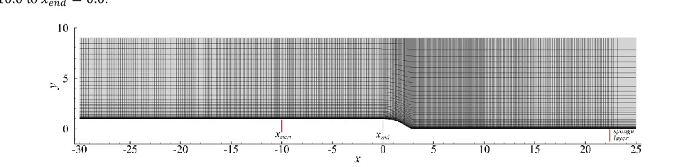
FIG. 1. The domain spans from x = -30.0 to 25.0 in the streamwise direction. A rounded ramp step of height H is attached to
the flat plate at x = 0.0. The SADS control is imposed onto the flat plate surface upstream of the rounded ramp from 𝑥𝑠𝑡𝑎𝑟𝑡 =
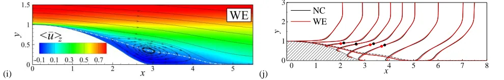
[image:7.612.64.544.298.416.2]−10.0 to 𝑥𝑒𝑛𝑑 = 0.0.
FIG. 1. Sketch of the computational domain and reduced numerical mesh. The mesh is plotted every 5th grid line in both x and y directions. A diagram showing the SADS control layout is illustrated in FIG. 2 (a). The active wall-normal velocity at the wall surface
imposed by the OPC and IPC, respectively, are given as
𝑣𝑤𝑎𝑙𝑙(𝑥, 𝑧) = −𝐴𝑂𝑃𝐶𝑣(𝑥, 𝑦𝑑𝑡𝑐, 𝑧) (7)
and
𝑣𝑤𝑎𝑙𝑙(𝑥, 𝑧) = +𝐴𝐼𝑃𝐶𝑣(𝑥, 𝑦𝑑𝑡𝑐, 𝑧) (8)
where 𝑣𝑤𝑎𝑙𝑙(𝑥, 𝑧) is the wall-normal velocity at the wall. The coefficients 𝐴𝑂𝑃𝐶 and 𝐴𝐼𝑃𝐶 are the two parameters that control
the amplitude of the wall velocity, which are both set to 0.5 in the present study to ensure the stability of the simulations. The
detected position in wall viscous units 𝑦𝑑𝑡𝑐+ , ranges from 12 (𝑥 = 𝑥𝑠𝑡𝑎𝑟𝑡) to 15 (𝑥 = 𝑥𝑒𝑛𝑑), for the baseline case. Choi et al. [51]
first introduced the OPC method into a turbulent channel flow where 𝐴𝑂𝑃𝐶 was set equal to 1.0. They observed a reduction in
skin friction of ~25% on each wall at 𝑦𝑑𝑡𝑐+ ≈ 10. Based on their study, Ni et al. [33,34] prescribed a fixed y-location of 𝑦𝑑𝑡𝑐+ ≈
11 in a SADS controlled turbulent channel flow, and their analysis suggested that the LSSVs can be generated and sustained
8
method is presented in FIG. 2b. Stroh et al. [22] studied the change of the secondary motion topology with the width of the
free-slip regions by restricting the spanwise wavelength of the no-slip/free-slip region. Similar to their parametric study, the
centre-to-centre spacing between two neighbouring OPC/IPC strips keep constant as the half of the computational domain
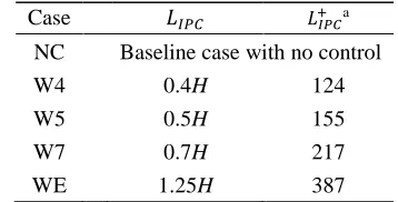
width 0.5𝐿𝑧, i.e. 𝐿𝐼𝑃𝐶+ 𝐿𝑂𝑃𝐶= 0.5𝐿𝑧. Four controlled cases with different IPC/OPC width are studied, and the widths of IPC
strips are summarised in TABLE I.
(a) (b)
FIG. 2. (a) Sketch of the topography configuration for equal spanwise width of OPC and IPC strips and (b) schematic of the control method used in the present study. The SADS control is imposed onto the flat plate surface upstream of the rounded ramp from 𝑥𝑠𝑡𝑎𝑟𝑡= −10.0 to
𝑥𝑒𝑛𝑑= 0.0. The regions of OPC and IPC are denoted by blue and red strips respectively in (a). The black and coloured arrows represent the
[image:8.612.73.543.181.297.2]wall-normal velocity at the detected position and the wall respectively in (b).
TABLE I. Summary of the ILES cases in the present study
Case 𝐿𝐼𝑃𝐶 𝐿𝐼𝑃𝐶+ a
NC Baseline case with no control
W4 0.4H 124
W5 0.5H 155
W7 0.7H 217
WE 1.25H 387
a 𝐿
𝐼𝑃𝐶
+ refers to 𝐿
𝐼𝑃𝐶 normalised by the wall viscous length scale of Case NC at 𝑥𝑠𝑡𝑎𝑟𝑡.
For all the cases studied, the reference Reynolds number is set to Re = 7,106. The Reynolds number based on nominal
thickness 𝛿, displacement thickness 𝛿∗ and momentum thickness 𝜃 of the boundary layer as well as the friction Reynolds
number 𝑅𝑒𝜏 at 𝑥 = 𝑥𝑠𝑡𝑎𝑟𝑡 are given in TABLE II. The reference Mach number is M = 0.2, defining a weakly compressible
boundary layer. The size of the computational domain in the streamwise and spanwise directions is 𝐿𝑥× 𝐿𝑧= 55 × 5 and for
the wall-normal direction, 𝐿𝑦 changes from 8 (upstream of the rounded ramp) to 9 (downstream of the rounded ramp). The
computational domain is discretised with a mesh of 1290 × 200 × 300 nodes in the streamwise, wall-normal and spanwise
directions, respectively. As shown in FIG. 1, the mesh is refined above the rounded ramp as well as its neighbouring upstream
and downstream regions along the streamwise direction, stretched towards the walls in the wall-normal direction and evenly
distributed in the spanwise direction. The mesh resolution at 𝑥 = 𝑥𝑠𝑡𝑎𝑟𝑡 in local wall unites is also presented in TABLE II.
[image:8.612.214.393.361.452.2]9
corresponds to ∆𝑡+= 3.2 × 10⁻³ normalised by the viscous time scale 𝑡
𝜏 =
𝑙𝜏
𝑢𝜏, where 𝑙𝜏= 𝜇𝑤
𝜌𝑤𝑢𝜏 is the wall viscous length
scale calculated by the wall units of the baseline case at 𝑥𝑠𝑡𝑎𝑟𝑡= −10.0.
TABLE II. Boundary layer parameters and mesh resolution at 𝑥 = 𝑥𝑠𝑡𝑎𝑟𝑡
x 𝑅𝑒𝛿a 𝑅𝑒𝛿∗ a 𝑅𝑒
𝜃 a 𝑅𝑒𝜏 b ∆𝑥+ ∆𝑦1+~∆𝑦𝛿+ ∆𝑧+
𝑥𝑠𝑡𝑎𝑟𝑡 14910 1715 1120 650 13.2 0.66~9.0 5.2
a 𝑅𝑒
𝛿, 𝑅𝑒𝛿∗ and 𝑅𝑒𝜃 refer to the Reynolds number based on nominal thickness 𝛿, displacement thickness 𝛿∗ and momentum thickness 𝜃,
respectively.
b The friction Reynolds number 𝑅𝑒
𝜏 is calculated via 𝑅𝑒𝜏= 𝜌𝑤𝑢𝜏𝛿
𝜇𝑤 based on the wall friction velocity 𝑢𝜏 at 𝑥𝑠𝑡𝑎𝑟𝑡, where 𝑢𝜏 is defined as
𝑢𝜏= √𝜌𝜏𝑤
𝑤, and 𝜏𝑤= 𝜇𝑤
𝜕𝑢
𝜕𝑦|𝑤 is the local wall shear stress.
A no-slip isothermal boundary condition is applied to the wall as 𝑇𝑤= 𝑇𝑟𝑒𝑓. The digital filter method proposed by Touber
and Sandham [54] is used to generate synthetic inflow turbulence and a transitional region of 18𝛿𝑠𝑡𝑎𝑟𝑡 is incorporated to let
synthetic fluctuations evolve into fully developed turbulence, where 𝛿𝑠𝑡𝑎𝑟𝑡 is the boundary-layer thickness at 𝑥 = 𝑥𝑠𝑡𝑎𝑟𝑡.
Morgan et al. [55] suggested that the flow reaches equilibrium status around 𝑥 𝛿⁄ 𝑟= 10.6 in a turbulent-boundary layer
developing over an adiabatic flat plate using digital filter method, where 𝛿𝑟 is the boundary-layer thickness at the reference
location. The generated artificial turbulent fluctuations are superimposed onto the turbulent mean velocity and temperature
profiles and introduced to the computational domain via the inflow boundary condition applied at 𝑥 = −30.0. At the upper and
outlet planes, generalised non-reflecting boundary conditions [56,57] are used. Sponge layers are applied at the outlet (𝑥 =
21.7) to filter the outgoing waves. Periodic boundary conditions are prescribed in the spanwise direction.
For the baseline case, after the transient period, the flow becomes fully turbulent and reaches a statistically steady state
after about 133 time units. After the imposition of the SADS control, the flow undergoes another transient period of around 70
time units before reaching a statistically steady state. For all the cases, the data samples are collected for at least 100 time units
before being post-processed and analyzed.
III. RESULTS AND DISCUSSIONS
In Section III.A, the results are first validated by comparing the baseline (denoted by Case NC) with the incompressible
DNS database of Schlatter and Örlü [58] and Jiménez et al. [60]. Then, the turbulence coherent structures visualised by the
iso-surfaces of the Q criterion are presented for all the cases in Section III.B to illustrate the impact of SADS control on the
turbulence intensity. It is followed by further analysis of the mean flow field data to study the influence of the strip width on
the mean statistics, including the skin friction coefficient Cf , the pressure coefficient Cp , the skin friction lines, the streamwise
10
the best control performance regarding the flow reattachment and the largest delay of the flow separation is obtained by Case
WE, and these two cases are analysed in detail in Section III.C.
A. Validation
To validate the numerical method, the mean velocity profile of the baseline case, normalised by the local friction velocity
𝑢𝜏 in the equilibrium zone (𝑥 = 𝑥𝑠𝑡𝑎𝑟𝑡), is compared with the classic law of the wall and the incompressible DNS data of
Schlatter and Örlü [58] in FIG. 3. In the present paper, "̅" and 〈 〉 stand for the time- and space-averaged operators,
respectively, i.e. 〈 〉𝑧 is used for the spanwise averaged variables. The fluctuations from each averaged operator are defined
as 𝑔′ = 𝑔 − 𝑔̅ and 𝑔〈𝑧〉= 𝑔 − 〈𝑔〉𝑧, where 𝑔 is a generic variable. The averaged operators can be combined as they are both
linear operators, i.e. 〈𝑔̅〉𝑧 and 𝑔′〈𝑧〉 might be used, for instance. According to FIG. 3, good agreement between the present ILES
result and the DNS data of Schlatter and Örlü [58] is obtained and the difference in the wake layer is attributed to Reynolds
number effects [59].
1 10 100 1000
0 5 10 15 20 25
DNS result from Schlatter and
Orlü at Re = 1000
Present ILES result at x = xstart
where Re = 1120
<u>
z
+
y+
u+=1/ κ·ln(y
+)+5.25
u
+=
y
+
··
FIG. 3. Mean velocity profile normalised by the local friction velocity. The von Kármán constant is κ=0.41.
The root mean square (RMS) velocity fluctuations 𝑢𝑖,𝑟𝑚𝑠′ = √〈𝑢̅̅̅̅̅̅̅̅̅̅̅̅〉𝑖,〈𝑧〉′ 𝑢𝑖,〈𝑧〉′ 𝑧 (i=1, 2, 3) and the Reynolds shear stress (RSS)
in the equilibrium zone of the baseline case are compared with the DNS data of Schlatter and Örlü [58] and Jiménez et al. [60]
in FIG. 4. A general good agreement for the RMS velocity fluctuations and the RSS are observed in the near-wall region.
However, high values of velocity fluctuations can be seen in the outer part of the boundary layer for the baseline case, which
is a common phenomenon observed in simulations of turbulent boundary layers using artificial inflow turbulence technologies
11
(a)
0 20 40 60 80 100
-1 0 1 2
3 ··
w'+rms
v'+ rms
u'+rms
DNS results from Schlatter and Orlü at Re=1000
DNS results from Jiménez et al.at Re=1100 Present ILES at x = xstart where Re=1120
y+ <u'<z>v'<z>>
+ z
(b)
0.0 0.5 1.0 1.5
-1 0 1 2 3
··
w'+rms
v'+rms u'
+ rms
DNS results from Schlatter and Orlü at Re = 1000 DNS results from Jiménez et al. at Re = 1100 Present ILES at x = xstart where Re = 1120
y/ <u'<z>v'<z>>
[image:11.612.68.546.54.235.2]+ z
FIG. 4. RMS velocity fluctuations and Reynolds shear stress in inner scaling (a) and outer scaling (b).
B. General Properties of the Flow Fields
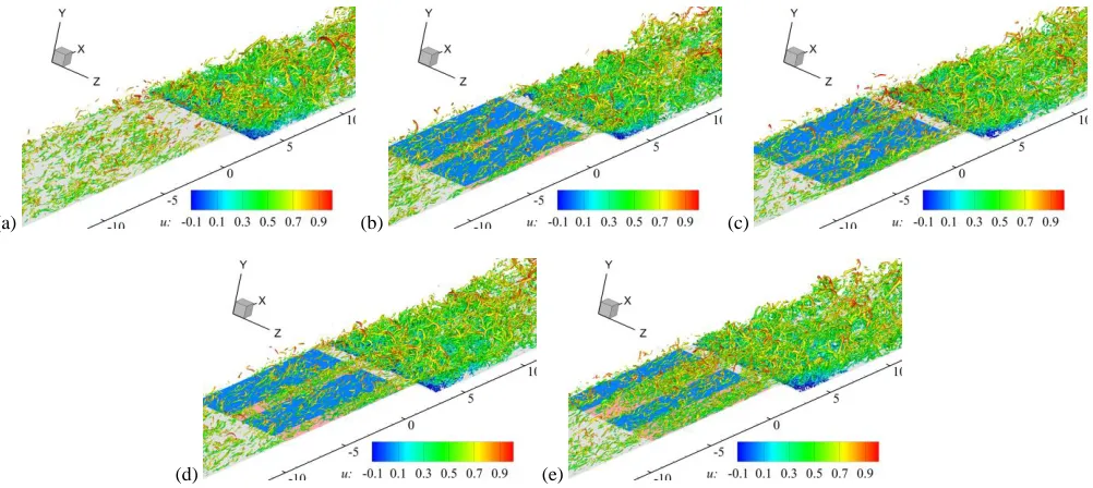
The turbulence coherent structures above the backward-facing rounded ramp and its neighbouring upstream and
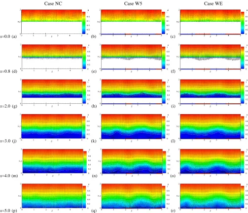
downstream regions, identified by the iso-surfaces of the Q criterion [62] (𝑄 = 4(𝑢𝑟𝑒𝑓⁄ )𝐻 2in FIG. 5) and coloured by the
instantaneous streamwise velocity u, are presented in FIG. 5 for all cases. Compared with the baseline case, the turbulence
coherent structures of cases with SADS are alternatively redistributed over the controlled region. In general, these turbulence
coherent structures are enhanced above the IPC strips, whereas above the OPC strips, a suppression of the coherent structures
can be observed. The flow field above the controlled zone demonstrates a phase-locked reorganisation in correspondence with
the topography configuration of the SADS distribution. The alternatively modified coherent structures above OPC/IPC strips
exhibit the same tendency as those in turbulent channel flows controlled by SADS [33,34], indicating the evidence of
suppression/enhancement of local turbulence. Furthermore, the alternating distributed suppressed and enhanced turbulence
coherent structures can extend to the downstream of the controlled area, which is more distinct in the case with wider width of
IPC strips (Case WE), as illustrated in FIG. 5 (c). More detailed quantitative analysis of the cases controlled by SADS will be
12
(a) (b) (c)
[image:12.612.59.560.51.275.2](d) (e)
FIG. 5. Turbulence coherent structures visualised with iso-surfaces of Q criterion and colored by instantaneous streamwise velocity u. The strips colored by blue and red on the wall upstream of the rounded ramp represent OPC and IPC regions respectively. (a) Case NC; (b) Case W4; (c) Case W5; (d) Case W7; (e) Case WE.
The mean statistics are analysed in detail in the following. The streamwise variation of the skin friction coefficient and
pressure coefficient are firstly dealt with based on their respective spanwise- and time-averaged statistics and presented in FIG.
6. The mean skin friction coefficient Cf and pressure coefficient Cp are defined as,
𝐶𝑓(𝑥) =
𝜇𝑤𝜕〈𝑢̅〉𝑧⁄𝜕𝑦|𝑤 1 2𝜌∞𝑢∞2
, (9)
and
𝐶𝑝(𝑥) =
〈𝑃̅〉𝑧−𝑃∞ 1 2𝜌∞𝑢∞2
. (10)
where the subscript “
∞
” refers to the incoming free-stream flow. It can be seen from FIG. 6 (a) that the near-wall flow upstreamof the rounded ramp undergoes an acceleration and thus the skin friction coefficient reaches a peak just before the rounded
ramp starts. This is due to the pressure drop induced by the convex curvature further downstream and the elliptic feature of the
pressure field [36], as shown in FIG. 6 (b). For the controlled cases, the SADS control causes an increase in the skin friction
upstream of the rounded ramp, due to the intense activation of turbulence locally by the IPC strip, which is consistent with the
previous studies of channel flow [33, 34]. Accordingly, the skin friction upstream of the rounded ramp for the controlled cases
increases with the width of the IPC strips monotonically. Case WE shows the highest skin friction upstream of the rounded
13
After reaching the rounded ramp, the flow decelerates because of the adverse pressure gradient and separation occurs. The
separation and reattachment locations, the length of the separation zone as well as the percentage reduction in the length of the
separation zone in comparison with the baseline case for all cases studied are summarised in TABLE III. It can be seen from
the zoomed left-hand-side sub-figure in FIG. 6 (a) and TABLE III that the time- and spanwise-averaged separation locations
for the cases with SADS control vary monotonically with the width of the IPC strips and the best performance with regards to
the separation delay is obtained by Case WE, whose IPC strips are the widest. It is because the enhanced turbulence above the
IPC strips goes downstream and then increases the momentum transport of the corresponding downstream region, leading to
the delay of separation. Since Case WE has the widest IPC strips among all the controlled cases, it leads to the biggest delay
of the separation point. This assumption can be verified in FIG. 7, which shows the contours of distance of the 𝑢̅ = 0 plane
projected onto the x-z surface. The white lines on the left-hand-side of the figures represent the separation lines while the
right-hand-side white lines refer to reattachment lines. The blue (resp. red) strips plotted beside the z-coordinate axis in FIG. 7
(b)-(e) represent the regions controlled by OPC (resp. IPC). It can be observed that the separation locations downstream of the IPC
strips are postponed whilst the separation positions are slightly shifted upstream in the limited regions downstream of the OPC
strips, thus leading to an overall delay of separation. It can also be seen from FIG. 7 (b)-(e) that the regions where the flow
separation is delayed are proportional to the width of the IPC strips. This is consistent with the separation locations summarised
in TABLE III that the largest separation delay is observed by Case WE, which has the widest width of the IPC strips. Further
downstream of the rounded ramp, the flow reattaches at x = 5.03 for the baseline case. However, after SADS control is imposed,
the flow shows a better performance regarding the reattachment location and Case W5 behaves the best among the four
controlled cases under consideration. The shortest length of separation zone is also achieved by Case W5 and the percentage
of reduction in the length of the separation zone in comparison with the baseline can be 8.49%, as shown in TABLE III. Since
much lower skin friction is induced by Case W5 upstream of the rounded ramp, it is the optimal one among all the cases studied
to suppress the flow separation. It can be seen from FIG. 6 (b) that there exists a pressure plateau within the separated
near-wall region for the baseline case whilst this plateau is lifted up after imposing SADS control, especially for Case WE. This
indicates that the control method adopted in the present study increases the pressure in the recirculation zone and plays a
14
(a)
-2 -1 0 1 2 3 4 5 6
-2 0 2 4 6 8 10
0.80 0.85 0.90
-0.5 0.0 0.5 1.0
4.6 4.7 4.8 4.9 5.0 5.1
-0.5 0.0 0.5 NC W4 W5 W7 WE Cf × 1 0 3
x (b)
-2 0 2 4 6 8
-0.3 -0.2 -0.1
0.0 NC
[image:14.612.70.556.55.201.2]W4 W5 W7 WE Cp x
FIG. 6. Skin friction coefficient Cf (a) and pressure coefficient Cp (b) based on spanwise- and time-averaged flow field. The grey line at the
[image:14.612.58.560.239.593.2]bottom of the figure and its underneath filled area represent the shape of the geometry adopted in the present study.
TABLE III. Summary of separation zone the characteristics regarding the flow separation and reattachment for all the cases
Case Separation location
Reattachment location
Length of the separation zone
Percentage of reduction in the length of the separation zone
NC 0.79 5.03 4.24 /
W4 0.82 4.85 4.03 4.95%
W5 0.84 4.72 3.88 8.49%
W7 0.86 4.88 4.02 5.19%
WE 0.92 4.83 3.91 7.78%
(a) (b) (c)
(d) (e)
FIG. 7. Distance between the contour line of the time-averaged streamwise velocity 𝑢̅ = 0 and the wall. The white lines on the left side of the figures show the separation lines while those right-hand-side white lines refer to reattachment lines. The blue and red strips plotted beside the z-coordinate axis in (b) and (c) represent the regions controlled by OPC and IPC respectively. The dash-dot lines divide the regions following the extension lines of the interface between the OPC and IPC strips upstream of the rounded ramp. (a) Case NC; (b) Case W4; (c) Case W5; (d) Case W7; (e) Case WE.
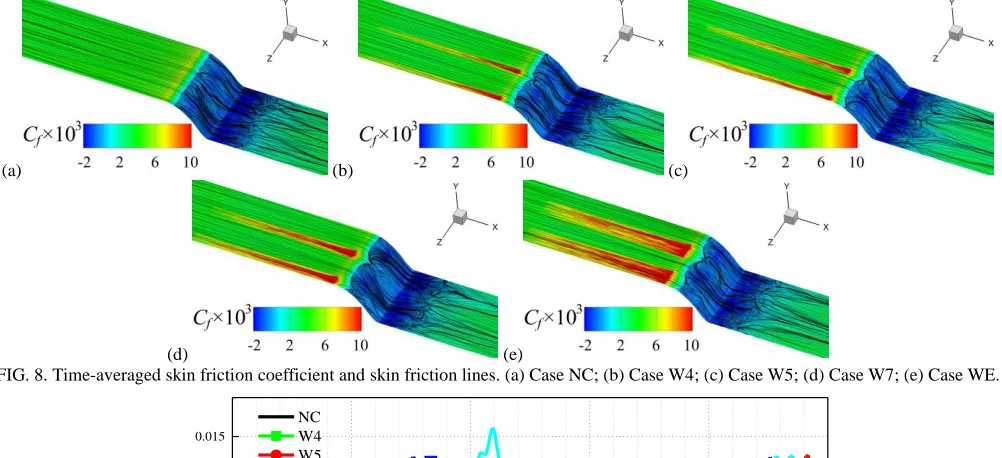
The distribution of the skin friction coefficient and the skin friction streamlines, for all the cases calculated by the
time-averaged statistics, are plotted in FIG. 8. In general, the skin friction coefficient increases over the IPC strips due to the increase
15
the rounded ramp are given in FIG. 9 to quantify the effect of both the OPC and IPC strips. It can be seen that the skin friction
coefficient is reduced over the OPC strips whereas it rises to a large extent over the IPC strips. Similar spanwise distribution
of the skin friction coefficient for the controlled cases was also observed in the SADS controlled turbulent channel flow [33,34].
However, a much more distinct decrease of the skin friction over the OPC strips is obtained compared with those in the channel
flow. A similar level of increase for all the controlled cases with regards to the spanwise-averaged value of 𝐶𝑓(𝑧)|𝑥=0.0above
the IPC strips can be seen in FIG. 9. This is independent of the IPC strip width and differs from the spanwise variation of the
skin friction coefficient in the SADS turbulent channel flow case where a clear maximum increase above the IPC strips is
obtained by the case with 2 pairs of equal-width strips (Case Nstrip4) [33], whose width is ∆𝑧+= 264 based on the friction
velocity of the baseline case. As reported by Mejia-Alvarez et al. [9], the abrupt wall stress variation would induce transverse
turbulent mixing which is the source of a 𝛿-scale secondary flow. Therefore, the spanwise heterogeneities of skin friction
generated by SADS control would induce large-scale streamwise structures. The skin friction lines for all the cases are plotted
in FIG. 8 to describe the 3-D flow structures. The critical point theory [63]focusing on the skin-friction lines can be used to
study 3-D structures near the reattachment locations. A critical point can be of three types: a node, saddle or focus. For the
controlled cases, a distinct node around the separation line can be observed downstream of the IPC strips whereas a saddle is
seen between the neighbouring nodes downstream of the OPC strips, as illustrated in FIG. 8 (b)-(e). The flow topology of the
controlled cases is reorganised by alternatively distributed OPC and IPC strips. It is shown in FIG. 8 (a) that 5 nodes around
the reattachment line can be recognized in Case NC whereas the number of the nodes in the corresponding region is reduced
to 4, 3, 4, 3 for Cases W4, W5, W7 and WE, respectively. It indicates that the spanwise spacing of the neighbouring nodes is
increased by SADS control, suggesting larger flow structures are dominating the flow reattachment. This should be the main
mechanism of the control method in improving the performance of flow reattachment. It can be seen that the number of the
nodes around the reattachment line in Cases W5 and WE is less than that in Cases W4 and W7, suggesting larger flow motions
are in the former two cases. Consequently, better control effects are obtained with regards to the reattachment locations, as
16
(a) (b) (c)
[image:16.612.57.558.56.285.2](d) (e)
FIG. 8. Time-averaged skin friction coefficient and skin friction lines. (a) Case NC; (b) Case W4; (c) Case W5; (d) Case W7; (e) Case WE.
0 1 2 3 4 5
0.005 0.010 0.015
NC W4 W5 W7 WE
z
Cf
(
z
)
|x=
0.0
FIG. 9. Mean skin friction coefficient 𝐶𝑓(𝑧)|𝑥=0.0 based on time-averaged statistics.
The distribution of the mean streamwise velocity 〈𝑢̅〉𝑧, normalised by the reference velocity 𝑢𝑟𝑒𝑓, obtained from the
turbulent boundary-layer flow upstream of the separation bubble through to the reattached flow region,are presented in FIG.
10. The zero-streamwise-velocity locations are shown as dash-dot white lines for all the cases on the left-hand-side of FIG. 10
whereas they are represented by dash-dot black line and solid red lines for the baseline case and the controlled cases,
respectively, on the right-hand-side of FIG. 10. The black and red solid circles in FIG. 10 (j) represent the inflection points of
the mean streamwise velocity profiles for the baseline case and the controlled case, respectively. These
zero-streamwise-velocity locations bisect the recirculation zone as mentioned in Bentaleb et al. [36]. Compared with Case NC, the SADS control
acts positively to suppress the flow separation for all cases.The size of the recirculation zone is reduced by SADS control
although the spanwise variation of the separation bubbles in the spanwise direction are enhanced, as indicated in FIG. 7
(b)-(e). It can be seen from FIG. 7 (b)-(e) that, for all the controlled cases, the height of the separation bubble downstream of the
IPC strips decreases whilst a relatively larger separation zone is obtained downstream of the OPC strips. Among all the
controlled cases, Case W5 shows a more effective influence on the second half of the recirculation zone and Case WE exhibits
17
2.0, 2.5, 3.0, 4.0, 5.0 and 5.5, are plotted on the right-hand-side of FIG. 10. This allows a quantitative comparison of the
evolution of the flow separation, reattachment and flow recovery to equilibrium status between the baseline case and the
controlled cases. It can be observed from Case WE (FIG. 10 (j)) that the near-wall flow is accelerated under the inflection point
of the velocity profile in the recirculation zone after imposing SADS control whereas the velocity in the outer part of the free
shear-layer slightly decreases compared with Case NC. This indicates that there exist large-scale structures in the controlled
case, which enhances the momentum transport between the main flow and the separated flow since the inflection point of the
streamwise velocity profile can be regarded as the edge of the recirculation zone. Therefore, the separated flow in the controlled
case has great potential to realise the reattachment shifting upstream. It can also be observed in FIG. 10 (j) that the inflection
points for Case WE shift towards the wall compared with those from the baseline case, demonstrating that the flow separation
is effectively suppressed by SADS control. Based on the above analysis, since Case W5 presents the best control performance
on the flow reattachment and the largest delay of the flow separation is obtained by Case WE, these two cases will be analysed
in detail.
(a) (b)
0 1 2 3
0 1 2 3 4 5 6 7 8
NC
x
y
(c) (d)
0 1 2 3
0 1 2 3 4 5 6 7 8
x
NC W4
y
(e) (f)
0 1 2 3
0 1 2 3 4 5 6 7 8
x
NC W5
y
(g) (h)
0 1 2 3
0 1 2 3 4 5 6 7 8
x
NC W7
18
(i) (j)
0 1 2 3
0 1 2 3 4 5 6 7 8
x
NC WE
[image:18.612.64.559.57.136.2]y
FIG. 10. Distribution of the mean streamwise velocity 〈𝑢̅〉𝑧 in outer scaling normalised by reference velocity (left-hand-side) and its profiles
at x = 0.0, 0.8, 1.5, 2.0, 2.5, 3.0, 4.0, 5.0 and 5.5 (right-hand-side). The zero-streamwise-velocity locations are shown as dash-dot white lines for all the cases on the left-hand-side whereas they are represented by dash-dot black line and solid red lines for the baseline case and the controlled cases, respectively, on the right-hand-side. The black and red solid circles in (j) represent the inflection points of the mean streamwise velocity profiles for the baseline case and the controlled case, respectively. The results come from Case NC, Case W4, Case W5, Case W7 and Case WE from top to bottom.
C. Comparative analysis of Cases NC, W5 and WE
a. Mean Flow
The mean streamwise velocity fields 𝑢̅in the y-z plane of Cases NC, W5 and WE selected from x = 0.0, 0.8, 2.0, 3.0, 4.0,
5.0 are compared in FIG. 11 to show the spanwise variation of the mean streamwise velocity in the separation zone. The
zero-streamwise-velocity locations are shown as dash-dot white lines for all the cases. The blue and red strips with black borders
plotted under the z-coordinate axis represent the corresponding regions downstream of the flat plate surface controlled by the
OPC and IPC strips, respectively. It can be seen from FIG. 11 (b) and (c) that the flow field at the beginning of the rounded
ramp (𝑥 = 0) is reorganized by Case W5 and WE compared with the baseline case in FIG. 11 (a). A transverse movement of
fluid is induced in the controlled cases between the neighbouring downstream of OPC and downstream of IPC strips. As
observed in FIG. 11 (e) and (f), around the separation point of Case NC, the near-wall velocity increases above the wall
downstream of IPC region whereas large-scale low-speed regions are induced above the wall downstream of OPC strips. The
accelerated fluid above the wall downstream of IPC regions play a critical role in delaying the flow separation as the ability of
the fluid to resist flow separation is enhanced. This has been verified in FIG. 7 (b) and (c) that flow above the wall downstream
of IPC regions separates later than that over the wall downstream of OPC strips. Therefore, a reasonable interpretation is that
the wider the IPC strips are, the better the delay of the flow separation works. This is also consistent with the mean separation
locations summarised in TABLE III, showing that Case WE exhibits the best separation delay. Further, it can be seen from
FIG. 11 (i), (l) and (o) that the height of the separation bubble is reduced above the wall downstream of IPC strips whereas in
the limited regions over the wall downstream of OPC strips, the recirculation zone enlarges in the wall-normal direction. This
suggests that the control method adopted in the present research takes a prominent role in suppressing flow separation. The
zero-streamwise-velocity locations calculated by time- and z-averaged statistics illustrated in FIG. 10 (f) show consistent results.
For Case W5 in the corresponding streamwise position (as indicated in FIG. 11 (h), (k) and (n)), the positive effects exerted on
19
downstream of IPC strips. This differs from the approximate phase-locked variation of the mean streamwise velocity imposed
by Case WE. In the reattachment region of Case WE, as indicated in FIG. 11 (q) and (r), spanwise alternating distributed low-
and high-velocity regions can be observed, similar to the observation in channel flow with SADS control [33,34]. Therefore,
the large-scale structures are induced by the alternating distributed OPC and IPC strips upstream of the rounded ramp, and they
can be sustained downstream of the rounded ramp and interact with the separation bubble and the reattachment flow.
Case NC Case W5 Case WE
x=0.0 (a) (b) (c)
x=0.8 (d) (e) (f)
x=2.0 (g) (h) (i)
x=3.0 (j) (k) (l)
x=4.0 (m) (n) (o)
[image:19.612.54.557.174.607.2]x=5.0 (p) (q) (r)
FIG. 11. Time-averaged streamwise velocity 𝑢̅ as well as mean velocity vector (𝑤̅, 𝑣̅) of Cases NC, W5 and WE from the left-hand-side to the right-hand-side respectively. The results come from x = 0.0, 0.8, 2.0, 3.0, 4.0 and 5.0 from top to bottom. The zero-streamwise-velocity locations are shown as dash-dot white lines for all the cases. The blue and red strips with black borders plotted under the z-coordinate axis represent the corresponding regions downstream of the flat plate surface controlled by the OPC and IPC strips respectively.
20
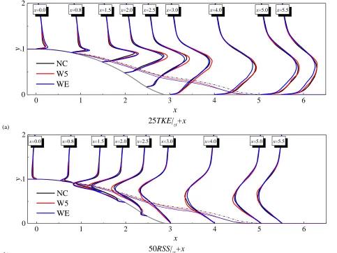
The TKE and RSS, normalised by square of the reference velocity, are presented in FIG. 12 at nine streamwise locations
ranging from x = 0.0 to x = 5.5 (before the detachment and after the reattachment). They are calculated with time- and z
-averaged statistics as,
𝑇𝐾𝐸|𝑧𝑡= 1
2〈(𝑢̅̅̅̅̅̅̅̅̅̅̅̅̅̅̅̅̅̅̅̅̅̅̅̅̅̅̅̅̅̅̅̅〉𝑘− 〈𝑢̅̅̅〉𝑘 𝑧)(𝑢𝑘− 〈𝑢̅̅̅〉𝑘 𝑧) 𝑧 𝑢𝑟𝑒𝑓 2
⁄ (𝑘 = 1,2,3) (11)
and
𝑅𝑆𝑆|𝑧𝑡= 〈(𝑢 − 〈𝑢̅〉𝑧̅̅̅̅̅̅̅̅̅̅̅̅̅̅̅̅̅̅̅̅̅̅̅̅̅̅〉)(𝑣 − 〈𝑣〉𝑧) 𝑧⁄𝑢𝑟𝑒𝑓2 (12)
where “ |𝑧𝑡” represents the fluctuation calculated by subtracting the z- and time-averaged velocity from the instantaneous one.
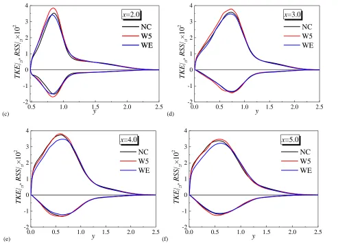
The distribution of the TKE|zt and RSS|ztat six representative streamwise positions (x = 0.0, 0.8, 2.0, 3.0, 4.0, 5.0) are zoomed
in FIG. 13. It can be seen from FIG. 12 (a) and FIG. 13 (a) that before the flow reaches the separation point, the TKE|zt of Cases
W5 and WE increase within the region of y = 1.6 in comparison with the baseline case. Between the two controlled cases, Case
WE exhibits a better performance in enhancing the near-wall turbulence energy, leading to a stronger extent of downstream
separation delay. In the outer part of the boundary layer (For Cases NC, W5 and WE, the local boundary-layer thickness is
comparable to the height of the rounded ramp.), a slight reduction of TKE|zt can be observed for both the controlled cases, and
a further loss in the wall-normal direction is seen in Case WE as more turbulence energy is transported into the near-wall region.
It can be seen that the variation of RSS|zt in FIG. 13 (a) is similar to that of TKE|zt.The similar distribution of TKE|zt and RSS|zt
for Cases NC, W5 and WE can be maintained until x = 1.5, as illustrated in FIG. 12. Higher levels of TKE|zt and RSS|zt have a
major contribution to the delay of flow separation. Inside the separation bubble, TKE|zt and RSS|zt are still higher for the
controlled cases at x = 2.0 due to the upstream effect. After flowing through the central part of the separated region (x = 3.0),
TKE|zt and RSS|zt of Case WE in the inner part of the boundary layer are gradually becoming smaller than those of Case NC,
but in the outer part of the boundary layer, both TKE|zt and RSS|zt are still higher than those of the non-controlled case, due to
the existence of LSSVs in the free shear-layer. Compared with Case WE, the RSS|zt of Case W5 still retains higher in the free
shear-layer, leading to a stronger momentum transport between the main flow and separated flow, and a faster flow
21
(a)
0
1
2
0
1
2
3
4
5
6
x=5.0 x=4.0 x=3.0 x=2.5 x=2.0 x=1.5 x=0.8
x=0.0 x=5.5
NC
W5
WE
25
TKE|
zt+x
x
y
(b) 0 1 20 1 2 3 4 5 6
NC
W5
WE
50
RSS|
zt+x
x
y
x=0.0 x=0.8 x=1.5 x=2.0 x=2.5 x=3.0 x=4.0 x=5.0 x=5.5
FIG. 12. (a) TKE and (b) RSS calculated by time- and z-averaged statistics for Cases NC, W5 and WE at x = 0.0, 0.8, 1.5, 2.0, 2.5, 3.0, 4.0, 5.0 and 5.5. The zero-streamwise-velocity locations are shown as a dash-dot black line, solid thin red and blue lines for Cases NC, W5 and WE respectively. Note that scaling multipliers are used to simply gain an equally clear view of the variations for all quantities.
(a)
1.0 1.5 2.0 2.5
0.0 0.5 1.0
TKE|
zt,
RSS|
zt×
10
2y
NC W5 WE x=0.0 (b)1.0 1.5 2.0 2.5
[image:21.612.70.553.56.419.2]22
(c)
0.5 1.0 1.5 2.0 2.5 -2 -1 0 1 2 3 4
TKE|
zt,
RSS|
zt×
10
2x
=2.0
NC
W5
WE
x
=2.0
NC
W5
WE
y
(d) 0.0 0.5 1.0 1.5 2.0 2.5-2 -1 0 1 2 3 4
TKE|
zt,
RSS|
zt×
10
2x
=3.0
NC
W5
WE
y
(e)0.0 0.5 1.0 1.5 2.0 2.5 -2 -1 0 1 2 3 4
TKE|
zt,
RSS|
zt×
10
2x
=4.0
NC
W5
WE
y
(f) 0.0 0.5 1.0 1.5 2.0 2.5-2 -1 0 1 2 3 4
TKE|
zt,
RSS|
zt×
10
2x
=5.0
NC
W5
WE
y
FIG. 13. TKE|zt and RSS|zt calculated by time- and z-averaged statistics for Cases NC, W5 and WE at x = 0.0, 0.8, 2.0, 3.0, 4.0 and 5.0,
respectively.
The distribution of TKE|t and RSS|t based on the time-averaged statistics as well as mean velocity vector (𝑤̅, 𝑣̅) at six
representative streamwise positions for Cases NC, W5 and WE are presented in FIG. 14 and FIG. 15 in order to further study
the properties of the LSSVs and the momentum transport. The definition of TKE|t and RSS|t is given as,
𝑇𝐾𝐸|𝑡=1 2𝑢𝑘
′𝑢 𝑘 ′
̅̅̅̅̅̅̅ 𝑢⁄ 𝑟𝑒𝑓2 (𝑘 = 1,2,3), (13)
[image:22.612.68.561.52.406.2]and
𝑅𝑆𝑆|𝑡= 𝑢̅̅̅̅̅̅ 𝑢𝑟𝑒𝑓′𝑣′⁄ 2 . (14)
Both TKE|t and RSS|t are normalised bythe square of the reference velocity 𝑢𝑟𝑒𝑓2 in Eqs. (13) and (14). “ |𝑡” expresses that the
fluctuation is calculated by subtracting the time-averaged velocity from the instantaneous one. It can be seen from FIG. 15
(a)-(c) that, compared with Case NC, the RSS|t of Cases W5 and WE are reorganised by the alternately distributed OPC and IPC
23
and thus a spanwise inhomogeneity of the Reynolds shear stress is induced. It can be seen from FIG. 14 (b) and (c) that more
turbulent energy is produced in the near-wall regions over the IPC strips following the spanwise variation of RSS|t. Fukagata
et al. [64] suggested that the Reynolds stress within 80 wall units from the wall is responsible for 90% of the turbulent
contribution to the total skin friction drag in a fully developed turbulent pipe flow. Choi et al. [51] utilised this to impose OPC
into a pipe flow to suppress the near-wall Reynolds stress, resulting in considerable drag reduction. Therefore, the enhanced
TKE and RSS above the IPC strips make major contributions to the total skin friction, which is consistent with the variation of
𝐶𝑓(𝑧)|𝑥=0.0shown in FIG. 9. A similar distribution of TKE|t and RSS|t for the controlled cases can be observed around the
separation location, as illustrated in the second rows of FIG. 14 and FIG. 15. As the near-wall turbulence is enhanced
downstream of IPC strips, the separation locations of Cases W5 and WE are delayed due to their ability to resist flow separation
improved. The control effect with regards to the separation delay is proportional to the width of the IPC strips upstream. This
is consistent with the mean separation locations of all the cases summarised in TABLE III. It can be seen from FIG. 14 and
FIG. 15 (g) that most of TKE is confined in the free shear-layer for the baseline case after the flow reaches the separated region.
However, for Cases W5 and WE, the TKE|t and RSS|t in the free shear-layer are redistributed by the sweep and ejection motions.
The sweep motions can be observed downstream of IPC as illustrated in FIG. 14 and FIG. 15 (h) and (i). They bring the high
momentum fluid from the free shear-layer into the separation bubble, leading to the high TKE|t and RSS|t obtained in the
near-wall region. The enhanced turbulent momentum transport results in the decrease of the height of the separation bubble as shown
by the solid black lines in FIG. 14 and FIG. 15 (h) and (i). It is worth mentioning that the reduction in the height of the separated
region is not limited to the regions downstream of the strips, especially for Case W5. It indicates that Case W5 exhibits a better
control effect with a narrower width of upstream IPC strips. On the other hand, the ejection motions take the low momentum
fluid from the inner part to the outer region of the separation bubble, enhancing the mixing procedure between the recirculation
region and the free shear-layer. Compared with Case WE, the TKE|t and RSS|t in the free shear-layer downstream of OPC strips
are enhanced by Case W5. In the further downstream region, a similar spanwise redistribution of the TKE|t and RSS|t in the
controlled cases can be observed throughout the whole separation regions, as illustrated in the fourth to fifth rows of FIG. 14
and FIG. 15. As reported by Le et al. [65], there exists an oscillatory large-scale roll-up of the shear-layer extending to the
reattachment region in the turbulent flow over a backward-facing step, leading to the motion of the reattachment location(s) in
the streamwise direction. Therefore, the large-scale structures generated by SADS control interact with the large-scale vortices
in the free shear-layer, leading to the reattachment locations being shifted upstream.Since the large-scale motions generated
by Case W5 have a relatively stronger impact on the distribution of TKE|t and RSS|t in the free shear-layer, the best control
24
reattachment regions, as observed in FIG. 14 and FIG. 15 (q) and (r). The spanwise distribution of alternating high-low TKE|t
and RSS|t streaks corresponds to the low-high mean streamwise velocity streaks in FIG. 10 (q) and (r), exhibiting that the
ejection and sweep motions are the major events related to the momentum transports. The penetration depth of the large-scale
motions displays the same order of magnitude as the local turbulent boundary-layer thickness.
Case NC Case W5 Case WE
x = 0.0 (a) (b) (c)
x = 0.8 (d) (e) (f)
x = 2.0 (g) (h) (i)
x = 3.0 (j) (k) (l)
x = 4.0 (m) (n) (o)
[image:24.612.52.561.155.595.2]x = 5.0 (p) (q) (r)
FIG. 14. TKE|t as well as mean velocity vector (𝑤̅, 𝑣̅)of Cases NC, W5 and WE from the left-hand-side to the right-hand-side respectively,
calculated by time-averaged statistics. The results come from x = 0.0, 0.8, 2.0, 3.0, 4.0, 5.0 from top to bottom. The zero-streamwise-velocity locations are shown as solid black lines for Cases NC, W5 and WE.
Case NC Case W5 Case WE
25
x = 0.8 (d) (e) (f)
x = 2.0 (g) (h) (i)
x = 3.0 (j) (k) (l)
x = 4.0 (m) (n) (o)
[image:25.612.55.560.53.398.2]x = 5.0 (p) (q) (r)
FIG. 15. RSS|t as well as mean velocity vector (𝑤̅, 𝑣̅) of Cases NC, W5 and WE from the left-hand-side to the right-hand-side respectively,
calculated by time-averaged statistics. The results come from x = 0.0, 0.8, 2.0, 3.0, 4.0 and 5.0 from top to bottom.
To highlight the variation of Reynolds stress in the spanwise direction, two other quantities, namely 〈(𝑢𝑖,〈𝑧〉′ − 𝑢 𝑖 ′)2〉
𝑧 and
〈(𝑢〈𝑧〉′ − 𝑢′)(𝑣 〈𝑧〉
′ − 𝑣′)〉
𝑧, are defined in Eqs. (15) and (16) to emphasize the influence of Cases W5 and WE on the modification
of the flow field in the spanwise direction,
〈(𝑢𝑖,〈𝑧〉′ − 𝑢 𝑖 ′)2〉
𝑧= 〈(𝑢𝑖̅ − 〈𝑢𝑖̅ 〉𝑧)2〉𝑧, (15)
and
〈(𝑢〈𝑧〉′ − 𝑢′)(𝑣
〈𝑧〉′ − 𝑣′)〉𝑧= 〈(𝑢̅ − 〈𝑢̅〉𝑧)(𝑣̅ − 〈𝑣̅〉𝑧)〉𝑧. (16)
The fluctuations are calculated by subtracting the z- and time-averaged velocity from the time-averaged one and i = 1,2,3 in
Eqs. (15) and (16). They are normalised bythe square of the reference velocity 𝑢𝑟𝑒𝑓2 as shown in the left-hand-side of FIG. 16
and 〈𝑢̅̅̅̅̅̅〉𝑖,〈𝑧〉′2
𝑧 (i =1,2,3) and 〈𝑢̅̅̅̅̅̅̅̅̅〉〈𝑧〉′ 𝑣〈𝑧〉′ 𝑧 (absolute value), respectively, as illustrated in the right-hand-side of FIG. 16. The results
come from x = 0.0, 0.8, 2.0, 3.0, 4.0 and 5.0. It can be seen from FIG. 16 (a) that, compared with Case NC, a doublet structure
of the streamwise normal stress is generated at x = 0.0 for Cases W5 and WE. The doublet positions locate at 0.011H (y+ = 5)
26
W5 and its outer peak is situated slightly away from the wall (0.092H, y+ = 35) in comparison with Case WE. As the new
definition of the Reynolds stress can exhibit the contribution of spanwise motions to the turbulent intensity by subtracting 〈𝑢̅〉𝑧
from 𝑢̅, we can infer that the doublet value of TKE is induced by the spanwise sharp inhomogeneous variation via alternately
distributed strips control in the spanwise direction. The inner peaks for the controlled cases are directly induced by the control
method itself. Further, the outer peak position is far away from the wall, indicating the existence of the large-scale motions
which should be the LSSVs generated in the logarithmic region of the turbulent boundary layer for the controlled cases. It is
worth mentioning that although the turbulent intensity around the inner peak in Case W5 is lower than that in Case WE, a
higher outer peak value is obtained in the former case. We assume that more intense large-scale structures are generated by
Case W5 and then interact with the downstream free shear-layer leading to a better performance with regards to the reattachment
point shifting upstream, as shown in TABLE III. The momentum transport of Cases W5 and WE are enhanced in the near-wall
region, leading to a significant rise of the streamwise component of turbulent intensity with a same peak position (inner peak)
compared to the Reynolds shear stress. The other two normal Reynolds stresses increase as well in comparison with those of
Case NC, as shown in FIG. 16 (a). Another normalisation using the local 〈𝑢̅̅̅̅̅̅〉𝑖,〈𝑧〉′2
𝑧 (i =1,2,3) and 〈𝑢̅̅̅̅̅̅̅̅̅〉〈𝑧〉′ 𝑣〈𝑧〉′ 𝑧 is presented in FIG.
16 (b). A doublet structure of the streamwise normal stress can also be observed. However, both the inner and outer peak values
of Case W5 are higher than those of Case WE, showing that Case W5 induces a relatively stronger spanwise inhomogeneity
with regards to the local Reynolds stresses in comparison with Case WE. Thus, it can be concluded that the large-scale
structures are generated by SADS control, and they play a significant role in the production of Reynolds stresses. Case W5 is
more efficient in creating large-scale structures, although Case WE produces more turbulent energy locally in the near-wall
region due to its wider IPC strips. Further, it can be seen from the left-hand-side of FIG. 16 that the large-scale spanwise
inhomogeneity induced by SADS control can be sustained in the downstream of separated region, even extending to the flow
recovery region (FIG. 16 (k)). The streamwise Reynolds normal stress and Reynolds shear stress in the controlled cases are
enhanced in comparison with Case NC. The near-wall peak of the streamwise Reynolds normal stress disappears over the
rounded ramp and the downstream reattachment region since the OPC and IPC strips are only imposed onto the flat plate
surface upstream of the rounded ramp. However, the outer peaks are maintained in the downstream region and situated around
the core of the free shear-layer. This indicates that the large-scale structures generated by SADS control can be sustained in the
downstream area and interact with the free shear-layer, leading to momentum transport enhancement and the reattachment
27
(a)
1.0 1.1 1.2 1.3
0.0 0.5 1.0 1.5
2.0
x
=0.0
NC W5 WE
streamwise normal stress
wall-normal normal stress
spanwise normal stress
shear stress
y
× 10 3 (b)1.0 1.1 1.2 1.3 1.4 1.5 -0.2
-0.1 0.0 0.1
0.2 NC W5 WE streamwise normal stress
wall-normal normal stress
spanwise normal stress
shear stress
x
=0.0
y
(c)
0.95 1.00 1.05
-2 0 2 4 6 8 × 10 3
x
=0.8
y
(d) 1.0 1.1 1.2-0.4 -0.2 0.0 0.2 0.4
x
=0.8
y
(e)0.6 0.8 1.0 1.2
-2 0 2 4 6 8 × 10 3
x
=2.0
y
(f) 0.6 0.8 1.0 1.2 1.4 1.6 1.8-0.2 -0.1 0.0 0.1
0.2
x
=2.0
28
(g)
0.0 0.2 0.4 0.6 0.8 1.0 1.2 1.4 1.6 -2 -1 0 1 2 3 4 5× 10 3
x
=3.0
y
(h) 0.0 0.5 1.0 1.5 2.0-3.0 -2.9 -0.2 -0.1 0.0 0.1 0.2
x
=3.0
y
(i)0.0 0.5 1.0 1.5
-2 -1 0 1 2 3 4 5× 10 3
x
=4.0
y
(j) 0.0 0.5 1.0 1.5 2.0-0.2 -0.1 0.0 0.1 0.2
x
=4.0
y
(k)0.0 0.2 0.4 0.6 0.8 1.0 1.2 1.4 1.6 -1 0 1 2 3 4 × 10 3
x
=5.0
y
(l) 0.0 0.5 1.0 1.5 2.0-0.1 0.0 0.1 0.2
x
=5.0
y
FIG. 16. Turbulent intensity 〈(𝑢𝑖,〈𝑧〉′ − 𝑢 𝑖′)
2
〉𝑧 and Reynolds shear stress 〈(𝑢〈𝑧〉′ − 𝑢′)(𝑣
〈𝑧〉′ − 𝑣′)〉𝑧 of Cases NC (line with symbols), W5
(solid lines) and WE (dash-dot lines) normalised by the square of the reference velocity 𝑢𝑟𝑒𝑓2 (left-hand-side) and 〈𝑢̅̅̅̅̅̅〉𝑖,〈𝑧〉′2 𝑧 (i =1,2,3) and
〈𝑢〈𝑧〉′ 𝑣 〈𝑧〉′
̅̅̅̅̅̅̅̅̅〉𝑧 (absolute value) respectively (right-hand-side). The definition of 〈(𝑢𝑖,〈𝑧〉′ − 𝑢𝑖′) 2
〉𝑧 and 〈(𝑢〈𝑧〉