Filter Design and Measurement Lab 08

ECE 300 Signals and Systems Fall 2009

Filter Design and Measurement

Lab 08

by Bruce A. Black, Robert Throne, and Mario Simoni

Objectives

In this lab we will examine filters in different ways. We will first investigate three different kinds of lowpass filters and the properties they possess. These filters illustrate the types of trade-offs we must make when designing a system. Finally we will determine the order of Butterworth filter we need to use to achieve a desired rejection.

Background

A periodic signal can be represented by the complex exponential form of the Fourier series. When a periodic signal is applied to the input of a filter, each of the harmonic components of the input signal experiences an amplitude and phase change caused by the filter. At the filter output the harmonic components add together to produce the output waveform. The amplitude and phase changes experienced by each of the input components combine to make the output signal different from the input signal in a predictable way. This difference between the input and output waveform is called distortion.

Stated mathematically, suppose x(t) is a periodic input signal with period T0, H(ω) is the frequency

response of the filter (i.e. the Fourier transform of its input response h(t)), and y(t) is the filter output. Then the input x(t) can be written

( )

0 0

, where 2 jk t

k k

x t a e ω ω π

∞

=−∞

=

∑

As the input signal passes through the filter, the input coefficients ak become altered by the filter to

become the output coefficients bk, where

(

)

k k

b =H kω a . The output y(t) is then given by

( )

(

)

0

jk t jk t

k k

k k

y t b e ω H kω a e ω

∞ ∞

=−∞ =−∞

=

∑

∑

Part 1: Filtering Periodic Signals

This is a continuation of the work you did in Lab 6. Now we are going to concentrate a bit more on the filters and examine some trade-offs between different common types of lowpass filters. Much of what follows is the same as for Lab 6, but there are a few changes at the end when we use different types of filters.

a) Use your code from Lab 6 to determine the Complex Fourier series representation using 20 terms of the following periodic function (defined over one period).

0 2

1 1 2

( )

3 2 3

0 3 4

t t x t t t 1

− ≤ < − ⎧

⎪ _{− ≤ <}

⎪

= ⎨ _{≤ <}

⎪

⎪ _{≤ <}

⎩

b) For the majority of the filters it uses, Matlab assumes filter has the form

1 2

1 2 1

1 2

1 2 1

( )

N N

N N

N N

N N

b s b s b s b s b

H s

a s a s a s a s a

− − − − 0 0 + + + + + = + + + + + " "

Hence, in order to represent any filter, Matlab just uses an array for the b coefficients and an array for the a coefficients. For example, we might have two variables (arrays) B and A to store the coefficients. These variables would be

[

]

[

]

B b b b

A a a

=

= a

Let’s assume we want to use a 10th order Butterworth lowpass filter with a frequency cutoff of 20ω₀. Use the help command to look up the Matlab function butter. You should return the coefficients in two arrays, i.e. your command should be [B,A] = butter(…..); Note that we are constructing an analog

filter here, so read all of the description for the butter command.

c) We now again need to find the variable H0 = H(0) and the variable (array)

[

]

H = H jω H j ω H jNω₀ . To find H(0) we use the fact that

0 0 (0) b H a =

If the b and a coefficients are stored in arrays B and A, we can write H0 = B(end)/A(end);

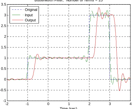
d) Plot the Fourier series representation for both the input signal x t( ) and the output signal on the same graph for N=25 terms, using different line types and a legend. The title of your graph should indicate that you are using a Butterworth filter. If you have done everything correctly your graph should look like that in Figure 1. Print out this graph and attach it to the worksheet at the end of this lab.

( ) y t

-2 -1 0 1 2 3 4

-1 -0.5 0 0.5 1 1.5 2 2.5 3 3.5

Time (sec)

Butterworth Filter, Number of Terms = 25

Original Input Output

Figure 1. Input and Fourier series representation of the input and output using a 10th order Butterworth filter.

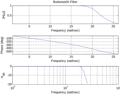
It will be useful to look at a frequency response plot of the filter you are using. You will need to make three plots on one page using the subplot command. Type orient tall before any of the plotting so you can use more of the page.

e) The first plot is the magnitude of the transfer function as a function of frequency. You will need to use the abs command. You should also put a grid on your figure.

f) The second plot is the phase of the transfer function (in degrees) as a function of frequency. In order to see the phenomena we want to see use the sequence of commands unwrap(angle(H))*180/pi. The most important command here is unwrap, which allows angles of more than 180 degrees

g) The third plot is the magnitude of the transfer function (in dB) as a function of frequency. Here you need to use the commands semilogx and log10.

5 10 15 20 25 0.5

1

Frequency (rad/sec)

|H(

ω

)|

Butterworth Filter

5 10 15 20 25

-500 -400 -300 -200 -100

Frequency (rad/sec)

P

h

as

e

(

d

eg

)

100 101 102

-20 -10 0

Frequency (rad/sec)

H dB

Figure 2. Frequency response of the 10th order Butterworth filter.

h) If the phase of the filter is exactly linear then we should have the relationship ( sec)

slope of filter in time delay

− =

Using a straight edge (or ruler), draw a line on your graph between the initial point on the phase graph and the value of the phase at about 20ω₀. Estimate the delay between the input and output signal (use Matlab to zoom in on the signal and measure this accurately, don’t just eyeball it!) and compare this to the predicted delay. Fill in the table on the worksheet.

i) Repeats parts b-h using a Bessel filter (use the command besself). Note that for this filter the frequency you specify can be considered the maximum frequency at which the phase will be linear.

Determine, by trial and error, the frequency you need to enter in order for the cutoff frequency to be at approximately 20ω_o. For this use multiples of ω_o, such as 30ω_o, 40ω_o, etc. Be sure to print out both graphs.

k) In the Chebyshev filter, try varying the R parameter from 0.5 (the default) to 2.0. What happens to the filter?

Part 2: Determining the Order of a Butterworth Filter

A Butterworth filter has the property that it is maximally flat in the passband. An nth order Butterworth filter has the magnitude squared response

2 2 1 | ( ) | 1 n p H ω ω ω = ⎛ ⎞ + ⎜_⎜ ⎟_⎟ ⎝ ⎠

where ω_pis the passband frequency. At this frequency the power has been reduced by one half or 3 dB, 2 2 1 1 | ( ) | 2 1 p n p p H ω ω ω = = ⎛ ⎞ + ⎜_⎜ ⎟_⎟ ⎝ ⎠

or 10 2 10

1 10 log | ( ) | 10 log 3

2 p

H ω = ⎛ ⎞_{⎜ ⎟}= d

⎝ ⎠ − B

To determine the required order of a filter we often look at the desired stopband frequency, ω_s. Usually we want to indicate the minimum required power difference between the passband and the stopband,Δ Δ. is the rejection.Hence we have

10 10

20 log |H(0) | 20 log |H(ω_s) |

Δ = −

or 10 2 1 10 log 1 n s p ω ω Δ = −

⎛ ⎞

+ ⎜_⎜ ⎟_⎟

⎝ ⎠

The ratio s p

ω

ω is called the transition ratio.

a) Show (on the back of the lab write-up) that we can write

10

ln 10 1

2 ln s p n ω ω Δ ⎛ ⎞ − ⎜ ⎟ ⎝ ⎠ = ⎛ ⎞ ⎜ ⎟ ⎜ ⎟ ⎝ ⎠

Note that n must be an integer, so we always round up (to the next larger integer).

Butterworth filter and verify that all frequencies ω ω> _s have magnitude (power) less than

.Matlab’s tf command and Bode commands will be really useful here. Note that you can click on the curve on the Bode plot to read it more accurately. Turn in your plot.

max Δ

c) For ω_p =15 rad/sec, ω_s =35rad/sec, and Δ =28 dB, determine the required Butterworth filter order for this filter. (Remember it must be an integer). Using Table 1, plot the Bode plot of your Butterworth filter and verify that all frequencies ω ω> _s have magnitude (power) less than Δ_max. Matlab’s tf

command and Bode commands will be really useful here. Turn in your plot.

2

3 2

4 3 2

5 4

denominator(s)

1 1

2 1.414 1

3 2 2 1

4 2.6131 3.4142 2.6131 1

5 3.2361 5

p

p p

p p p

p p p p

p p

n

s

s s

s s s

s s s s

s s

ω

ω ω

ω ω ω

ω ω ω ω

ω ω

+

⎛ ⎞ ⎛ ⎞

+ +

⎜ ⎟ ⎜ ⎟

⎜ ⎟ ⎜ ⎟

⎝ ⎠ ⎝ ⎠

⎛ ⎞ ⎛ ⎞ ⎛ ⎞

+ + +

⎜ ⎟ ⎜ ⎟ ⎜ ⎟

⎜ ⎟ ⎜ ⎟ ⎜ ⎟

⎝ ⎠ ⎝ ⎠ ⎝ ⎠

⎛ ⎞ ⎛ ⎞ ⎛ ⎞ ⎛ ⎞

+ + + +

⎜ ⎟ ⎜ ⎟ ⎜ ⎟ ⎜ ⎟

⎜ ⎟ ⎜ ⎟ ⎜ ⎟ ⎜ ⎟

⎝ ⎠ ⎝ ⎠ ⎝ ⎠ ⎝ ⎠

⎛ ⎞ ⎛ ⎞

+ +

⎜ ⎟ ⎜ ⎟

⎜ ⎟ ⎜ ⎟

⎝ ⎠ ⎝ ⎠

3 2

.2361 5.2361 3.2361 1

p p p

s

s s

ω ω ω

⎛ ⎞ ⎛ ⎞ ⎛ ⎞

+ + +

⎜ ⎟ ⎜ ⎟ ⎜ ⎟

⎜ ⎟ ⎜ ⎟ ⎜ ⎟

⎝ ⎠ ⎝ ⎠ ⎝ ⎠

Lab 08

Instructor Verification Sheet

Name___________________________Date:___________

At the end of this lab you should have attached the following plots:

• Two plots for the Butterworth filter (input/output and transfer function characteristics)

• Two plots for the Bessel filter

• Two plots for the Chebyshev filter

• One plot for part 2-b (Butterworth Order)

• One plot for part 2-c (Butterworth Order)

Part1: Measurements of Different Filters

Filter Type

Predicted Delay (-slope of filter)

Measured Delay (time domain) 10th order Butterworth

10th order Bessel 10th order Chebyshev

Question 1: From Part 1, which filter type has the most linear phase over the passband? This filter will have the smallest phase distortion.

Question 2: From Part 1, which filter has the flattest magnitude response over the passband? This filter will have the smallest magnitude distortion.

Question 3: From Part 1, which filter has the steepest rolloff after the cutoff frequency ?