ISSN Online: 2161-7198 ISSN Print: 2161-718X
DOI: 10.4236/ojs.2018.86059 Dec. 4, 2018 885 Open Journal of Statistics
Linear Regression Analysis
for Symbolic Interval Data
Jin-Jian Hsieh, Chien-Cheng Pan
Department of Mathematics, National Chung Cheng University, Taiwan
Abstract
In the network technology era, the collected data are growing more and more
complex, and become larger than before. In this article, we focus on estimates
of the linear regression parameters for symbolic interval data. We propose
two approaches to estimate regression parameters for symbolic interval data
under two different data models and compare our proposed approaches with
the existing methods via simulations. Finally, we analyze two real datasets
with the proposed methods for illustrations.
Keywords
Linear Regression, Symbolic Interval Data, Centre Method, Least Squares
Estimate
1. Introduction
In classical statistical analysis, the collected data usually have exact value. But, in
network technology era, the collected data are usually symbolic type. Diday [1]
in-troduced symbolic data which are presented in the form of intervals, histograms,
lists and so on. Unlike the classical data, symbolic data could be presented in more
types in a p-dimensional space
p. We discuss symbolic interval data in this
ar-ticle, which are symbolic interval-values no longer an exact value. With this
change, the classical methods may not be available. Therefore, it is necessary to
develop new methods for the analysis of symbolic data. With covariates, we
study parameter estimates of the linear regression for symbolic interval data.
Billard and Diday [2] used the center point of each interval-value to fit the
li-near regression model. Carvalho
et al.
[3] used the center point and range of
each interval-value to fit two linear regression models. Xu [4] used the symbolic
covariance method for the symbolic interval data, which was introduced by
Bil-How to cite this paper: Hsieh, J.-J. and Pan, C.-C. (2018) Linear Regression Analy-sis for Symbolic Interval Data. Open Jour-nal of Statistics, 8, 885-901.
https://doi.org/10.4236/ojs.2018.86059
Received: October 24, 2018 Accepted: December 1, 2018 Published: December 4, 2018
Copyright © 2018 by authors and Scientific Research Publishing Inc. This work is licensed under the Creative Commons Attribution International License (CC BY 4.0).
http://creativecommons.org/licenses/by/4.0/
DOI: 10.4236/ojs.2018.86059 886 Open Journal of Statistics
lard [5]. In this article, we present two approaches to estimate regression
para-meters for symbolic interval data. The first method considers the endpoints least
square estimate, and the second method considers the least squares estimate
with interval weighted function.
This paper is organized as follows. Section 2 gives a introduction for symbolic
interval data, Model 1 and Model 2. In Section 3, we propose two methods to
es-timate regression coefficient for symbolic interval data. In Section 4, the
com-parisons of the proposed methods and some existing methods are performed via
simulations. In Section 5, we analyze two real datasets with the proposed
ap-proaches. Finally, we make some concluding remarks in Section 6.
2. Data and Models
2.1. Symbolic Interval Data
In this article, we study on symbolic regression of interval-valued data. First of
all, we introduce the symbolic interval data. In classical data, the exact value of
the interested variables usually can be observed. In the network technology era,
the collected data are growing more and more complex, and no longer a single
point. Diday [1] introduced the new data format which is called as symbolic data.
Symbolic data have several types as follows: intervals, histograms, lists and so on. For
the several types, it is necessary to develop some new methods. For example, because
of privacy issues, we usually cannot collect the exact data from respondents. Thus,
we usually design some questionnaires to collect the symbolic interval data. For
no-tations, define
X
ij=
a b Y
ij,
ij
,
i=
[
c d i
i,
i]
,
=
1, , ,
n j
=
1, ,
p
.
(
Y
1, ,
Y
n)
′
=
Y
,
X
i=
(
X
i1, ,
X
ip)
′
and
X
=
(
X
1′
, ,
X
n′
)
′
. Thus, the observed
data are
{
(
Y X
i,
i1, ,
X
ip)
:
i
=
1, ,
n
}
.
2.2. Model 1
This model considered the linear regression model for symbolic interval data as
0 1 1
,
i i p ip i
Y
=
β
+
β
X
+
+
β
X
+
ε
(1)
0 1 1
0 1 1
,
i U p ipU iU iU
i L p ipL iL iL
X
X
Y
X
X
Y
β
β
β
ε
β
β
β
ε
+
+ +
+
⇔
=
+
+ +
+
(2)
where
i
=
1, ,
n
,
(
β
1, ,
β
p)
are the parameters of interest, and
ε
iis the
error term. Here, we assume
X
ijL<
X
ijU, which is also considered by Billard and
Diday [2]. Therefore,
a
ij=
X
ijLand
b
ij=
X
ijU. Due to the unknown of β's, we
cannot identify the order of
Y
iLand
Y
iU. Hence,
Y
iUis either
c
ior
d
i, and
the remaining one is
Y
iL. This model implies that the length of
Y
idepends on
the lengths of
X
i. But, in practice, the length of
Y
imay not depends on
lengths of
X
i. Thus, we also consider the different model, Model 2.
2.3. Model 2
DOI: 10.4236/ojs.2018.86059 887 Open Journal of Statistics
* * *
0 1 1
,
1, , ,
i i p ip i
Y
=
β β
+
X
+ +
β
X
+
ε
i
=
n
(3)
where
*i
Y
and
*ij
X
are single points,
(
β
1, ,
β
p)
are the parameters of
inter-est, and
ε
iis the error term. In practice,
(
Y X
i*,
ij*)
may not be observed due to
privacy issues or some reasons. Usually, the proxies
Y
i=
[
c d
i,
i]
,
X
ij=
a b
ij,
ij
of
(
*,
*)
i ij
Y X
can be collected. Note that
*i i
Y
∈
Y
and
*ij ij
X
∈
X
,
i
=
1, ,
n
,
1, ,
j
=
p
. Thus, the collected data is
{
(
Y X
i,
i1, ,
X
ip)
:
i
=
1, ,
n
}
. In this
model, the length of
Y
idoes not depend on the lengths of
X
i.
3. The Proposed Estimations
3.1. Method 1: Endpoints Least Squares Estimate
Based on Model 1, we propose the endpoints least squares estimation approach
to estimate
(
β
0, ,
β
p)
. We assume that
X
ijL<
X
ijU,
i
=
1, ,
n
,
j
=
1, ,
p
,
which is also considered by Billard and Diday [2]. Due to the unknown of
β′
is
,
the order of
(
Y Y
iL,
iU)
cannot be identified. We consider the following
proce-dure to identify the order of
(
Y Y
iL,
iU)
. From model 1, the model is presented as
follows,
0 1 1 2 2
0 1 1 2 2
,
,
iU i U i U p ipU iU
iL i L i L p ipL iL
Y
X
X
X
Y
X
X
X
β
β
β
β
ε
β
β
β
β
ε
=
+
+
+ +
+
=
+
+
+ +
+
(4)
where
i
=
1, ,
n
. To identify the order of
Y
iLand
Y
iU, we apply the centre
method [2] to obtain the estimates of
β
as
β
ˆ
c.
Then, compute
ˆ
c iUY
and
ˆ
c iLY
as
0 1 1 2 2
0 1 1 2 2
ˆ
ˆ
ˆ
ˆ
ˆ
,
ˆ
ˆ
ˆ
ˆ
ˆ
.
c c c c c
iU i U i U p ipU
c c c c c
iL i L i L p ipL
Y
X
X
X
Y
X
X
X
β
β
β
β
β
β
β
β
=
+
+
+ +
=
+
+
+ +
(5)
When
ˆ
cˆ
c iL iUY
<
Y
,
Y
iL=
c
iand
Y
iU=
d
i. When
Y
ˆ
iUc<
Y
ˆ
iLc,
Y
iU=
c
iand
iL i
Y
=
d
. Then we would obtain the estimates of
β
by the endpoints least
squares estimate as
(
)
(
)
1 1ˆ
,
ˆ
,
U U U U U
L L L L L
− −
′
′
=
′
′
=
X X
X Y
X X
X Y
β
β
(6)
where
Y
U=
(
Y
1U, ,
Y
nU)
′
,
Y
L=
(
Y
1L, ,
Y
nL)
′
,
X
U=
(
X
1U, ,
X
nU)
′
,
(
1, ,
)
L L nL
X
=
X
X
′
,
X
iU=
(
X
i U1, ,
X
ipU)
and
X
iL=
(
X
i L1, ,
X
ipL)
. Then,
set
ˆ
ˆ
ˆ
.
2
U
+
L=
β
β
β
(7)
ˆ
β
is the estimator of
β
in model 1.
3.2. Method 2: Interval Weighted Least Squares Estimate
The method 2 is provided for the model 2, which allows the length of
Y
idoes
not depend on the lengths of
X
i. The centre method [2] estimates the
in-DOI: 10.4236/ojs.2018.86059 888 Open Journal of Statistics
terval data. Based on the centre method [2], we think the lengths of the interval
data can provide some different information in the estimation procedure.
Therefore, we use the lengths of the interval data to construct some weighted
functions, which provide different impact for each data observation in least
squares estimation procedure. Denote the weighted function by
ki
W
. Thus, we
suggest the interval weighted least squares estimation method as
(
)
2*
0 1 1 2 2 1
min
n c c c c,
i i i i p ip
i
W Y
X
X
X
β
β
β
β
=
−
−
−
− −
∑
β
(8)
where
*1
n
k k
i i i
i
W
W
W
=
=
∑
,
i
=
1, ,
n
,
k
=
1,2,3
. As the results of (8), the
mini-mizer
β
ˆ
is the estimator of
β
in model 2. Through some examinations in
simulations, we suggest three weighted functions of the length of the interval
data in the following. Denote the length of interval:
ri i i
Y
=
d c
−
,
rij ij ij
X
=
b a
−
,
( )
max
r r
i i
MY
=
Y
and
rmax
( )
r j i ijMX
=
X
,
i
=
1, ,
n
,
j
=
1, ,
p
. The first
weighted function is designed as
1 * * * *
1 1 1 1
1
exp
ir pexp
ijr,
i r r
j j
X
Y
W
a b
c d
MY
=MX
=
+ ×
−
+
+
×
−
∑
(9)
where
i
=
1, ,
n
and
* * * * 1, , ,
1 1 1a b c d
are positive constants. The weighted
func-tion is exponential decline as the lengths of interval data increasing. The second
weighted function is given as
2 * * * *
2 2 2 2
1
,
r r p ij ii r r
j j
X
Y
W
a b
c d
MY
=MX
=
+ × −
+
+
× −
∑
(10)
where
i
=
1, ,
n
,
* * * * 2, , ,
2 2 2a b c d
are positive constants,
* * 2 2b
<
a
and
* * 2 2d
<
c
.
The weighted function is linear decline as the lengths of interval data increasing.
Define the standardized lengths of interval data
ir rY
MY
and
r ij r j
X
MX
as
SY
irand
r ijSX
. Let
1
n1 r i iSY
n
∑
=and
11
n rij i
SX
n
∑
=be
rSY
and
r jSX
. The third
weighted function is designed as
1 3 * 3 * * 3 3 1 * 3 * *
1 3 3
1 exp
2
2
1 exp
2
,
2
r r i i r r p ij j jSY
SY
W
a
a
a
SX
SX
a
a
a
− − =
−
=
−
−
−
+
−
−
∑
(11)
where
i
=
1, ,
n
and
* 3DOI: 10.4236/ojs.2018.86059 889 Open Journal of Statistics
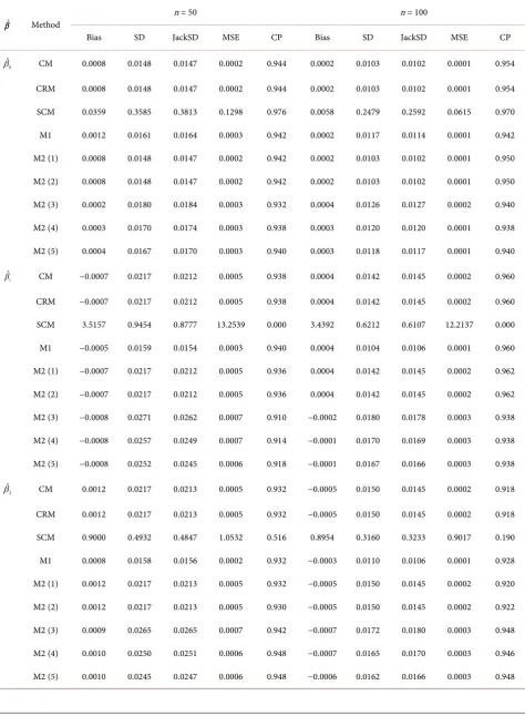
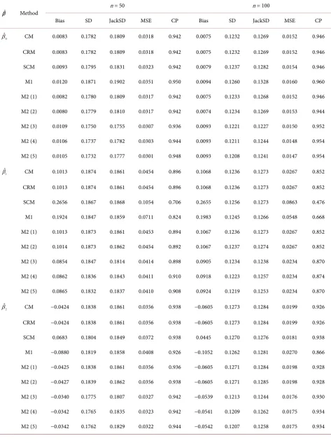
4. Simulation
In this section, we compare our proposed methods, endspoints least squares
estimator (M1) and interval weighted least squares estimator (M2), with the
existing methods, CM [2], CRM [3] and SCM [4], by simulated datasets. We
consider two data generations for model 1 and model 2. For each table, we
present the bias, empirical standard deviation (SD), average of jackknife
stan-dard deviation (JackSD), mean squares error (MSE), and 95% coverage
proba-bility (CP). Data are simulated with sample size n = 50 and 100, and
replica-tions R = 500.
For model 1: we first generate 2 independent values from
(
0,
2)
jX
N
σ
, and let
ijU
X
be the larger one and
X
ijLbe the smaller one, where
i
=
1, ,
n
,
j
=
1,2
.
The error term
~
(
0,
2)
L
iL
N
εε
σ
and
~
(
0,
2)
U
iU
N
εε
σ
,
i
=
1, ,
n
. Then, we
generate
Y
iLand
Y
iUas
0 1 1 2 2
0 1 1 2 2
,
.
iL i L i L iL
iU i U i U iU
Y
X
X
Y
X
X
β
β
β
ε
β
β
β
ε
=
+
+
+
=
+
+
+
(12)
The
β
=
(
β β β
0, ,
1 2)
are set as
(
10,10,5
)
and
(
10, 10,5
−
)
.
(
1 2)
2
,
2,
2,
2L U
X X ε ε
σ σ
σ σ
are set as
(
1,1,0.1,0.1
)
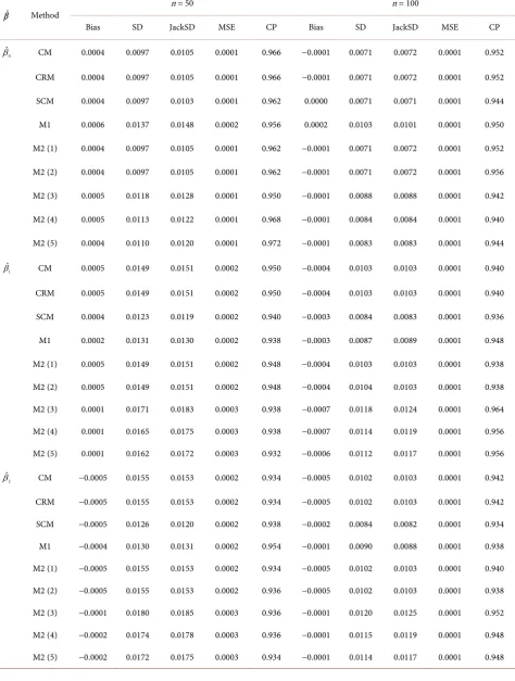
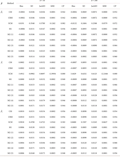
. In Table 1 & Table 2, we consider
the interval data have the same error terms of
(
Y Y
iL,
iU)
. That is,
(
)
~
0,0.1
iL iU
N
ε
=
ε
. In Table 3 &
Table 4, we consider the error terms of
(
Y Y
iL,
iU)
are different. That is,
ε
iL~
N
(
0,0.1
)
and
ε
iU~
N
(
0,0.1
)
. From the
results, the endpoints least squares estimation (M1) has smaller standard
devia-tion than others for
β
1and
β
2under Table 1, Table 2 and Table 4. SCM has
better performance than others under Table 3. Note that SCM has poor
perfor-mance when
(
β β β =
1, ,
2 3) (
10, 10,5
−
)
in Table 2 and Table 4.
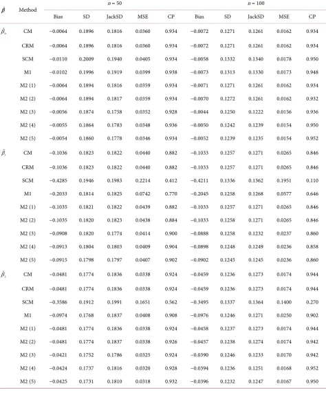
For model 2: we first generate the single points
*~
(
0,
2)
jij X
X
N
σ
,
j
=
1,2
,
(
2)
~
0,
i
N
εε
σ
and set
* * *
0 1 1 2 2
,
i i i i
Y
=
β
+
β
X
+
β
X
+
ε
(13)
where
i
=
1, ,
n
. To construct the interval data, the range is generated from a
uniform distribution, and denote the upper range of
(
*,
*)
i ij
Y X
by
(
h,
h)
iU ijUY X
and the lower range of
(
*,
*)
i ij
Y X
by
(
h,
h)
iL ijLY X
,
i
=
1, ,
n
,
j
=
1,2
. Therefore,
we could built the interval-valued data as
[
,
]
* h,
* hi i i iL i iU
c d
=
Y Y Y
−
+
Y
and
* *
,
h,
hij ij ij ijL ij ijU
a b
X
X X
X
=
−
+
,
i
=
1, ,
n
,
j
=
1,2
. Thus, we obtain the
in-terval data
(
Y X X
i,
i1,
i2)
,
i
=
1, ,
n
. For the settings,
β
=
(
β β β
0, ,
1 2)
are set
as
(
10,10,5
)
and
(
10, 10,5
−
)
, and
(
2,
2)
j
X ε
σ
σ
are set as
(
1,0.5
)
,
j
=
1,2
.
h iLY
,
h iU
Y
,
h ijLX
and
h ijUX
are generated from uniform distribution such as
h iLY
and
h iU
Y
from
U
( )
0,
b
1h,
X
i Lh1and
X
i Uh1from
U
( )
0,
b
2h, and
X
i Lh2and
X
i Uh2from
U
( )
0,
b
3h,
i
=
1, ,
n
. Note that M2 (1) is the interval weighted LSE with the
first weighted function, W
1, and
(
* * * *)
(
)
1
, , ,
1 1 11,0.2,1,0.15
a b c d
=
; M2 (2) is the
me-thod with the second weighted function, W
2, and
(
* * * *)
(
)
2
, , ,
2 2 21,0.2,1,0.15
a b c d
=
;
M2 (3) is the method with the third weighted function, W
3, and
* 30.5
a
=
; M2 (4)
is the method with the third weighted function, W
3, and
*3
1
DOI: 10.4236/ojs.2018.86059 890 Open Journal of Statistics
Table 1. Estimations of
β
under model 1 with(
β β β =0, ,1 2) (
10,10,5)
.ˆ
β Method n = 50 n = 100
Bias SD JackSD MSE CP Bias SD JackSD MSE CP
0
ˆ
β CM −0.0014 0.0139 0.0146 0.0002 0.966 0.0008 0.0100 0.0102 0.0001 0.952
CRM −0.0014 0.0139 0.0146 0.0002 0.966 0.0008 0.0100 0.0102 0.0001 0.952
SCM −0.0014 0.0138 0.0144 0.0002 0.964 0.0008 0.0099 0.0101 0.0001 0.954
M1 −0.0011 0.0160 0.0163 0.0003 0.944 0.0008 0.0113 0.0114 0.0001 0.944
M2 (1) −0.0014 0.0139 0.0146 0.0002 0.966 0.0008 0.0100 0.0102 0.0001 0.954
M2 (2) −0.0014 0.0139 0.0146 0.0002 0.966 0.0008 0.0100 0.0102 0.0001 0.954
M2 (3) −0.0007 0.0173 0.0182 0.0003 0.946 0.0006 0.0119 0.0126 0.0001 0.968
M2 (4) −0.0007 0.0165 0.0173 0.0003 0.942 0.0007 0.0114 0.0120 0.0001 0.964
M2 (5) −0.0007 0.0162 0.0170 0.0003 0.944 0.0007 0.0112 0.0118 0.0001 0.964
1
ˆ
β CM −0.0011 0.0215 0.0214 0.0005 0.934 0.0005 0.0149 0.0146 0.0002 0.950
CRM −0.0011 0.0215 0.0214 0.0005 0.934 0.0005 0.0149 0.0146 0.0002 0.950
SCM −0.0009 0.0162 0.0162 0.0003 0.938 0.0003 0.0115 0.0112 0.0001 0.950
M1 −0.0007 0.0156 0.0156 0.0002 0.934 0.0003 0.0109 0.0107 0.0001 0.952
M2 (1) −0.0011 0.0215 0.0214 0.0005 0.934 0.0005 0.0149 0.0146 0.0002 0.948
M2 (2) −0.0011 0.0215 0.0214 0.0005 0.934 0.0005 0.0150 0.0146 0.0002 0.948
M2 (3) −0.0018 0.0255 0.0269 0.0007 0.944 0.0001 0.0183 0.0179 0.0003 0.930
M2 (4) −0.0017 0.0244 0.0256 0.0006 0.944 0.0002 0.0174 0.0171 0.0003 0.930
M2 (5) −0.0017 0.0241 0.0252 0.0006 0.940 0.0002 0.0171 0.0168 0.0003 0.938
2
ˆ
β CM 0.0011 0.0206 0.0212 0.0004 0.946 0.0006 0.0151 0.0145 0.0002 0.936
CRM 0.0011 0.0206 0.0212 0.0004 0.946 0.0006 0.0151 0.0145 0.0002 0.936
SCM 0.0010 0.0157 0.0161 0.0002 0.952 0.0004 0.0116 0.0112 0.0001 0.932
M1 0.0008 0.0151 0.0154 0.0002 0.950 0.0004 0.0110 0.0106 0.0001 0.932
M2 (1) 0.0011 0.0206 0.0212 0.0004 0.948 0.0006 0.0152 0.0145 0.0002 0.938
M2 (2) 0.0011 0.0207 0.0212 0.0004 0.950 0.0007 0.0152 0.0145 0.0002 0.942
M2 (3) 0.0003 0.0254 0.0262 0.0006 0.946 0.0004 0.0189 0.0178 0.0004 0.922
M2 (4) 0.0005 0.0243 0.0251 0.0006 0.946 0.0004 0.0181 0.0170 0.0003 0.920
DOI: 10.4236/ojs.2018.86059 891 Open Journal of Statistics
Table 2. Estimations of
β
under model 1 with(
β β β =0, ,1 2) (
10, 10,5−)
.ˆ
β Method
n = 50 n = 100
Bias SD JackSD MSE CP Bias SD JackSD MSE CP
0
ˆ
β CM 0.0008 0.0148 0.0147 0.0002 0.944 0.0002 0.0103 0.0102 0.0001 0.954
CRM 0.0008 0.0148 0.0147 0.0002 0.944 0.0002 0.0103 0.0102 0.0001 0.954
SCM 0.0359 0.3585 0.3813 0.1298 0.976 0.0058 0.2479 0.2592 0.0615 0.970
M1 0.0012 0.0161 0.0164 0.0003 0.942 0.0002 0.0117 0.0114 0.0001 0.942
M2 (1) 0.0008 0.0148 0.0147 0.0002 0.942 0.0002 0.0103 0.0102 0.0001 0.950
M2 (2) 0.0008 0.0148 0.0147 0.0002 0.942 0.0002 0.0103 0.0102 0.0001 0.950
M2 (3) 0.0002 0.0180 0.0184 0.0003 0.932 0.0004 0.0126 0.0127 0.0002 0.940
M2 (4) 0.0003 0.0170 0.0174 0.0003 0.938 0.0003 0.0120 0.0120 0.0001 0.938
M2 (5) 0.0004 0.0167 0.0170 0.0003 0.940 0.0003 0.0118 0.0117 0.0001 0.940
1
ˆ
β CM −0.0007 0.0217 0.0212 0.0005 0.938 0.0004 0.0142 0.0145 0.0002 0.960
CRM −0.0007 0.0217 0.0212 0.0005 0.938 0.0004 0.0142 0.0145 0.0002 0.960
SCM 3.5157 0.9454 0.8777 13.2539 0.000 3.4392 0.6212 0.6107 12.2137 0.000
M1 −0.0005 0.0159 0.0154 0.0003 0.940 0.0004 0.0104 0.0106 0.0001 0.960
M2 (1) −0.0007 0.0217 0.0212 0.0005 0.936 0.0004 0.0142 0.0145 0.0002 0.962
M2 (2) −0.0007 0.0217 0.0212 0.0005 0.936 0.0004 0.0142 0.0145 0.0002 0.962
M2 (3) −0.0008 0.0271 0.0262 0.0007 0.910 −0.0002 0.0180 0.0178 0.0003 0.938
M2 (4) −0.0008 0.0257 0.0249 0.0007 0.914 −0.0001 0.0170 0.0169 0.0003 0.938
M2 (5) −0.0008 0.0252 0.0245 0.0006 0.918 −0.0001 0.0167 0.0166 0.0003 0.938
2
ˆ
β CM 0.0012 0.0217 0.0213 0.0005 0.932 −0.0005 0.0150 0.0145 0.0002 0.918
CRM 0.0012 0.0217 0.0213 0.0005 0.932 −0.0005 0.0150 0.0145 0.0002 0.918
SCM 0.9000 0.4932 0.4847 1.0532 0.516 0.8954 0.3160 0.3233 0.9017 0.190
M1 0.0008 0.0158 0.0156 0.0002 0.932 −0.0003 0.0110 0.0106 0.0001 0.928
M2 (1) 0.0012 0.0217 0.0213 0.0005 0.932 −0.0005 0.0150 0.0145 0.0002 0.920
M2 (2) 0.0012 0.0217 0.0213 0.0005 0.930 −0.0005 0.0150 0.0145 0.0002 0.922
M2 (3) 0.0009 0.0265 0.0265 0.0007 0.942 −0.0007 0.0172 0.0180 0.0003 0.948
M2 (4) 0.0010 0.0250 0.0251 0.0006 0.948 −0.0007 0.0165 0.0170 0.0003 0.946
DOI: 10.4236/ojs.2018.86059 892 Open Journal of Statistics
Table 3. Estimations of
β
under model 1 with(
β β β =0, ,1 2) (
10,10,5)
.ˆ
β Method n = 50 n = 100
Bias SD JackSD MSE CP Bias SD JackSD MSE CP
0
ˆ
β CM 0.0004 0.0097 0.0105 0.0001 0.966 −0.0001 0.0071 0.0072 0.0001 0.952
CRM 0.0004 0.0097 0.0105 0.0001 0.966 −0.0001 0.0071 0.0072 0.0001 0.952
SCM 0.0004 0.0097 0.0103 0.0001 0.962 0.0000 0.0071 0.0071 0.0001 0.944
M1 0.0006 0.0137 0.0148 0.0002 0.956 0.0002 0.0103 0.0101 0.0001 0.950
M2 (1) 0.0004 0.0097 0.0105 0.0001 0.962 −0.0001 0.0071 0.0072 0.0001 0.952
M2 (2) 0.0004 0.0097 0.0105 0.0001 0.962 −0.0001 0.0071 0.0072 0.0001 0.956
M2 (3) 0.0005 0.0118 0.0128 0.0001 0.950 −0.0001 0.0088 0.0088 0.0001 0.942
M2 (4) 0.0005 0.0113 0.0122 0.0001 0.968 −0.0001 0.0084 0.0084 0.0001 0.940
M2 (5) 0.0004 0.0110 0.0120 0.0001 0.972 −0.0001 0.0083 0.0083 0.0001 0.944
1
ˆ
β CM 0.0005 0.0149 0.0151 0.0002 0.950 −0.0004 0.0103 0.0103 0.0001 0.940
CRM 0.0005 0.0149 0.0151 0.0002 0.950 −0.0004 0.0103 0.0103 0.0001 0.940
SCM 0.0004 0.0123 0.0119 0.0002 0.940 −0.0003 0.0084 0.0083 0.0001 0.936
M1 0.0002 0.0131 0.0130 0.0002 0.938 −0.0003 0.0087 0.0089 0.0001 0.948
M2 (1) 0.0005 0.0149 0.0151 0.0002 0.948 −0.0004 0.0103 0.0103 0.0001 0.938
M2 (2) 0.0005 0.0149 0.0151 0.0002 0.948 −0.0004 0.0104 0.0103 0.0001 0.938
M2 (3) 0.0001 0.0171 0.0183 0.0003 0.938 −0.0007 0.0118 0.0124 0.0001 0.964
M2 (4) 0.0001 0.0165 0.0175 0.0003 0.938 −0.0007 0.0114 0.0119 0.0001 0.956
M2 (5) 0.0001 0.0162 0.0172 0.0003 0.932 −0.0006 0.0112 0.0117 0.0001 0.956
2
ˆ
β CM −0.0005 0.0155 0.0153 0.0002 0.934 −0.0005 0.0102 0.0103 0.0001 0.942
CRM −0.0005 0.0155 0.0153 0.0002 0.934 −0.0005 0.0102 0.0103 0.0001 0.942
SCM −0.0005 0.0126 0.0120 0.0002 0.938 −0.0002 0.0084 0.0082 0.0001 0.934
M1 −0.0004 0.0130 0.0131 0.0002 0.954 −0.0001 0.0090 0.0088 0.0001 0.938
M2 (1) −0.0005 0.0155 0.0153 0.0002 0.934 −0.0005 0.0102 0.0103 0.0001 0.940
M2 (2) −0.0005 0.0155 0.0153 0.0002 0.936 −0.0005 0.0102 0.0103 0.0001 0.938
M2 (3) −0.0001 0.0180 0.0185 0.0003 0.936 −0.0001 0.0120 0.0125 0.0001 0.952
M2 (4) −0.0002 0.0174 0.0178 0.0003 0.936 −0.0001 0.0115 0.0119 0.0001 0.948
DOI: 10.4236/ojs.2018.86059 893 Open Journal of Statistics
Table 4. Estimations of
β
under model 1 with(
β β β =0, ,1 2) (
10, 10,5−)
.ˆ
β Method n = 50 n = 100
Bias SD JackSD MSE CP Bias SD JackSD MSE CP
0
ˆ
β CM −0.0002 0.0106 0.0104 0.0001 0.942 −0.0004 0.0069 0.0072 0.0000 0.952
CRM −0.0002 0.0106 0.0104 0.0001 0.942 −0.0004 0.0069 0.0072 0.0000 0.952
SCM 0.0191 0.3548 0.3789 0.1262 0.982 −0.0132 0.2404 0.2588 0.0579 0.972
M1 −0.0006 0.0151 0.0147 0.0002 0.936 −0.0003 0.0093 0.0101 0.0001 0.960
M2 (1) −0.0002 0.0106 0.0104 0.0001 0.940 −0.0004 0.0069 0.0072 0.0000 0.952
M2 (2) −0.0002 0.0106 0.0104 0.0001 0.940 −0.0004 0.0069 0.0072 0.0000 0.952
M2 (3) 0.0000 0.0121 0.0130 0.0001 0.950 −0.0004 0.0089 0.0090 0.0001 0.964
M2 (4) 0.0000 0.0116 0.0123 0.0001 0.946 −0.0003 0.0084 0.0084 0.0001 0.962
M2 (5) 0.0000 0.0114 0.0120 0.0001 0.946 −0.0003 0.0082 0.0083 0.0001 0.960
1
ˆ
β CM 0.0002 0.0152 0.0152 0.0002 0.932 −0.0007 0.0093 0.0103 0.0001 0.962
CRM 0.0002 0.0152 0.0152 0.0002 0.932 −0.0007 0.0093 0.0103 0.0001 0.962
SCM 3.4912 0.8982 0.8697 12.9956 0.000 3.4429 0.6252 0.6125 12.2446 0.000
M1 0.0000 0.0129 0.0132 0.0002 0.940 −0.0009 0.0080 0.0088 0.0001 0.972
M2 (1) 0.0002 0.0153 0.0152 0.0002 0.932 −0.0007 0.0093 0.0103 0.0001 0.966
M2 (2) 0.0002 0.0153 0.0152 0.0002 0.930 −0.0007 0.0092 0.0103 0.0001 0.966
M2 (3) 0.0000 0.0183 0.0188 0.0003 0.948 −0.0008 0.0120 0.0128 0.0001 0.956
M2 (4) 0.0001 0.0174 0.0179 0.0003 0.946 −0.0008 0.0112 0.0121 0.0001 0.956
M2 (5) 0.0001 0.0171 0.0175 0.0003 0.944 −0.0008 0.0110 0.0118 0.0001 0.958
2
ˆ
β CM 0.0010 0.0151 0.0154 0.0002 0.956 −0.0003 0.0098 0.0103 0.0001 0.954
CRM 0.0010 0.0151 0.0154 0.0002 0.956 −0.0003 0.0098 0.0103 0.0001 0.954
SCM 0.9018 0.4700 0.4722 1.0342 0.502 0.8680 0.3307 0.3245 0.8627 0.228
M1 0.0006 0.0130 0.0133 0.0002 0.942 −0.0003 0.0085 0.0089 0.0001 0.954
M2 (1) 0.0010 0.0151 0.0154 0.0002 0.958 −0.0003 0.0098 0.0103 0.0001 0.956
M2 (2) 0.0010 0.0151 0.0154 0.0002 0.958 −0.0003 0.0098 0.0103 0.0001 0.956
M2 (3) 0.0004 0.0179 0.0184 0.0003 0.944 −0.0005 0.0120 0.0127 0.0001 0.968
M2 (4) 0.0005 0.0171 0.0176 0.0003 0.948 −0.0005 0.0114 0.0120 0.0001 0.960
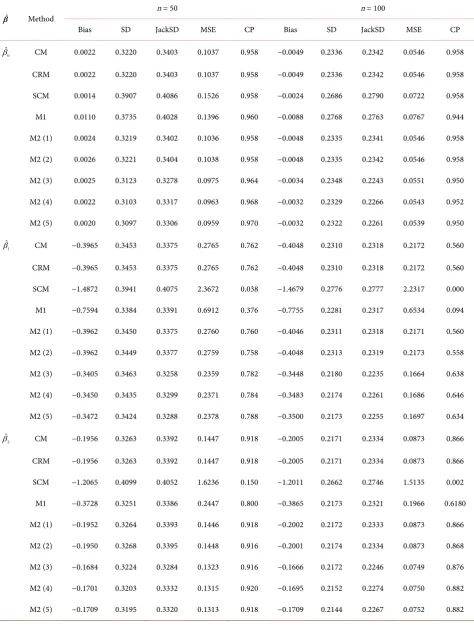
DOI: 10.4236/ojs.2018.86059 894 Open Journal of Statistics
method with the third weighted function, W
3, and
*3
2
[image:10.595.63.538.155.730.2]a
=
. The simulation
re-sults are shown in Tables 5-8. From the rere-sults, the interval weighted least
squares estimation with W
3has better performance than others.
Table 5. Estimations of
β
under model 2 with(
β β β =0, ,1 2) (
10,10,5)
, and b1h=b2h=b3h=0.5.ˆ
β Method n = 50 n = 100
Bias SD JackSD MSE CP Bias SD JackSD MSE CP
0
ˆ
β CM −0.0064 0.1896 0.1816 0.0360 0.934 −0.0072 0.1271 0.1261 0.0162 0.934
CRM −0.0064 0.1896 0.1816 0.0360 0.934 −0.0072 0.1271 0.1261 0.0162 0.934
SCM −0.0110 0.2009 0.1940 0.0405 0.934 −0.0058 0.1332 0.1340 0.0178 0.950
M1 −0.0102 0.1996 0.1919 0.0399 0.938 −0.0073 0.1313 0.1330 0.0173 0.948
M2 (1) −0.0064 0.1894 0.1816 0.0359 0.934 −0.0071 0.1271 0.1261 0.0162 0.934
M2 (2) −0.0064 0.1894 0.1817 0.0359 0.934 −0.0070 0.1272 0.1261 0.0162 0.932
M2 (3) −0.0056 0.1874 0.1758 0.0352 0.928 −0.0044 0.1250 0.1222 0.0156 0.936
M2 (4) −0.0055 0.1864 0.1783 0.0348 0.936 −0.0050 0.1242 0.1239 0.0154 0.950
M2 (5) −0.0054 0.1860 0.1778 0.0346 0.934 −0.0052 0.1239 0.1235 0.0154 0.952
1
ˆ
β CM −0.1036 0.1823 0.1822 0.0440 0.882 −0.1033 0.1257 0.1271 0.0265 0.846
CRM −0.1036 0.1823 0.1822 0.0440 0.882 −0.1033 0.1257 0.1271 0.0265 0.846
SCM −0.4285 0.1946 0.1983 0.2214 0.412 −0.4211 0.1336 0.1362 0.1951 0.110
M1 −0.2033 0.1814 0.1825 0.0742 0.770 −0.2045 0.1258 0.1268 0.0577 0.646
M2 (1) −0.1035 0.1821 0.1822 0.0439 0.882 −0.1033 0.1257 0.1271 0.0265 0.846
M2 (2) −0.1035 0.1820 0.1823 0.0438 0.884 −0.1033 0.1258 0.1271 0.0265 0.846
M2 (3) −0.0908 0.1820 0.1774 0.0414 0.900 −0.0888 0.1258 0.1232 0.0237 0.860
M2 (4) −0.0913 0.1804 0.1803 0.0409 0.904 −0.0898 0.1248 0.1249 0.0236 0.858
M2 (5) −0.0915 0.1798 0.1797 0.0407 0.902 −0.0902 0.1245 0.1245 0.0236 0.860
2
ˆ
β CM −0.0481 0.1774 0.1836 0.0338 0.924 −0.0459 0.1236 0.1273 0.0174 0.944
CRM −0.0481 0.1774 0.1836 0.0338 0.924 −0.0459 0.1236 0.1273 0.0174 0.944
SCM −0.3586 0.1912 0.1991 0.1651 0.562 −0.3495 0.1337 0.1364 0.1400 0.270
M1 −0.0974 0.1768 0.1837 0.0408 0.908 −0.0976 0.1246 0.1271 0.0250 0.902
M2 (1) −0.0481 0.1774 0.1836 0.0338 0.924 −0.0458 0.1237 0.1273 0.0174 0.944
M2 (2) −0.0481 0.1774 0.1837 0.0338 0.926 −0.0457 0.1238 0.1274 0.0174 0.942
M2 (3) −0.0421 0.1752 0.1786 0.0325 0.924 −0.0390 0.1246 0.1233 0.0170 0.942
M2 (4) −0.0424 0.1737 0.1816 0.0320 0.928 −0.0394 0.1236 0.1251 0.0168 0.952
DOI: 10.4236/ojs.2018.86059 895 Open Journal of Statistics Table 6. Estimations of
β
under model 2 with(
β β β =0, ,1 2) (
10, 10,5−)
, and b1h=b2h=b3h=0.5.ˆ
β Method n = 50 n = 100
Bias SD JackSD MSE CP Bias SD JackSD MSE CP
0
ˆ
β CM 0.0083 0.1782 0.1809 0.0318 0.942 0.0075 0.1232 0.1269 0.0152 0.946
CRM 0.0083 0.1782 0.1809 0.0318 0.942 0.0075 0.1232 0.1269 0.0152 0.946
SCM 0.0093 0.1795 0.1831 0.0323 0.942 0.0079 0.1237 0.1282 0.0154 0.946
M1 0.0120 0.1871 0.1902 0.0351 0.950 0.0094 0.1260 0.1328 0.0160 0.960
M2 (1) 0.0082 0.1780 0.1809 0.0317 0.942 0.0075 0.1233 0.1268 0.0152 0.946
M2 (2) 0.0080 0.1779 0.1810 0.0317 0.942 0.0074 0.1234 0.1269 0.0153 0.944
M2 (3) 0.0109 0.1750 0.1755 0.0307 0.936 0.0093 0.1221 0.1227 0.0150 0.952
M2 (4) 0.0106 0.1737 0.1782 0.0303 0.944 0.0093 0.1211 0.1244 0.0148 0.954
M2 (5) 0.0105 0.1732 0.1777 0.0301 0.948 0.0093 0.1208 0.1241 0.0147 0.954
1
ˆ
β CM 0.1013 0.1874 0.1861 0.0454 0.896 0.1068 0.1236 0.1273 0.0267 0.852
CRM 0.1013 0.1874 0.1861 0.0454 0.896 0.1068 0.1236 0.1273 0.0267 0.852
SCM 0.2656 0.1867 0.1868 0.1054 0.706 0.2655 0.1256 0.1273 0.0863 0.476
M1 0.1924 0.1847 0.1859 0.0711 0.824 0.1983 0.1245 0.1266 0.0548 0.668
M2 (1) 0.1013 0.1873 0.1861 0.0453 0.894 0.1067 0.1236 0.1273 0.0267 0.852
M2 (2) 0.1014 0.1873 0.1862 0.0454 0.892 0.1067 0.1237 0.1274 0.0267 0.852
M2 (3) 0.0854 0.1847 0.1814 0.0414 0.898 0.0905 0.1234 0.1238 0.0234 0.870
M2 (4) 0.0862 0.1836 0.1843 0.0411 0.910 0.0918 0.1223 0.1257 0.0234 0.874
M2 (5) 0.0865 0.1832 0.1837 0.0410 0.908 0.0924 0.1219 0.1253 0.0234 0.870
2
ˆ
β CM −0.0424 0.1838 0.1861 0.0356 0.938 −0.0605 0.1273 0.1284 0.0199 0.926
CRM −0.0424 0.1838 0.1861 0.0356 0.938 −0.0605 0.1273 0.1284 0.0199 0.926
SCM 0.0683 0.1804 0.1849 0.0372 0.938 0.0445 0.1270 0.1276 0.0181 0.938
M1 −0.0880 0.1819 0.1858 0.0408 0.926 −0.1052 0.1262 0.1281 0.0270 0.866
M2 (1) −0.0425 0.1838 0.1861 0.0356 0.936 −0.0605 0.1271 0.1284 0.0198 0.928
M2 (2) −0.0427 0.1839 0.1862 0.0356 0.938 −0.0605 0.1271 0.1285 0.0198 0.928
M2 (3) −0.0340 0.1775 0.1807 0.0327 0.942 −0.0539 0.1213 0.1244 0.0176 0.930
M2 (4) −0.0342 0.1765 0.1835 0.0323 0.942 −0.0541 0.1209 0.1262 0.0175 0.934
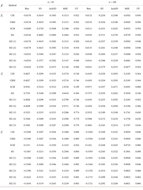
DOI: 10.4236/ojs.2018.86059 896 Open Journal of Statistics Table 7. Estimations of
β
under model 2 with(
β β β =0, ,1 2) (
10,10,5)
, and b1h=b2h=b3h=1.ˆ
β Method n = 50 n = 100
Bias SD JackSD MSE CP Bias SD JackSD MSE CP
0
ˆ
β CM 0.0022 0.3220 0.3403 0.1037 0.958 −0.0049 0.2336 0.2342 0.0546 0.958
CRM 0.0022 0.3220 0.3403 0.1037 0.958 −0.0049 0.2336 0.2342 0.0546 0.958
SCM 0.0014 0.3907 0.4086 0.1526 0.958 −0.0024 0.2686 0.2790 0.0722 0.958
M1 0.0110 0.3735 0.4028 0.1396 0.960 −0.0088 0.2768 0.2763 0.0767 0.944
M2 (1) 0.0024 0.3219 0.3402 0.1036 0.958 −0.0048 0.2335 0.2341 0.0546 0.958
M2 (2) 0.0026 0.3221 0.3404 0.1038 0.958 −0.0048 0.2335 0.2342 0.0546 0.958
M2 (3) 0.0025 0.3123 0.3278 0.0975 0.964 −0.0034 0.2348 0.2243 0.0551 0.950
M2 (4) 0.0022 0.3103 0.3317 0.0963 0.968 −0.0032 0.2329 0.2266 0.0543 0.952
M2 (5) 0.0020 0.3097 0.3306 0.0959 0.970 −0.0032 0.2322 0.2261 0.0539 0.950
1
ˆ
β CM −0.3965 0.3453 0.3375 0.2765 0.762 −0.4048 0.2310 0.2318 0.2172 0.560
CRM −0.3965 0.3453 0.3375 0.2765 0.762 −0.4048 0.2310 0.2318 0.2172 0.560
SCM −1.4872 0.3941 0.4075 2.3672 0.038 −1.4679 0.2776 0.2777 2.2317 0.000
M1 −0.7594 0.3384 0.3391 0.6912 0.376 −0.7755 0.2281 0.2317 0.6534 0.094
M2 (1) −0.3962 0.3450 0.3375 0.2760 0.760 −0.4046 0.2311 0.2318 0.2171 0.560
M2 (2) −0.3962 0.3449 0.3377 0.2759 0.758 −0.4048 0.2313 0.2319 0.2173 0.558
M2 (3) −0.3405 0.3463 0.3258 0.2359 0.782 −0.3448 0.2180 0.2235 0.1664 0.638
M2 (4) −0.3450 0.3435 0.3299 0.2371 0.784 −0.3483 0.2174 0.2261 0.1686 0.646
M2 (5) −0.3472 0.3424 0.3288 0.2378 0.788 −0.3500 0.2173 0.2255 0.1697 0.634
2
ˆ
β CM −0.1956 0.3263 0.3392 0.1447 0.918 −0.2005 0.2171 0.2334 0.0873 0.866
CRM −0.1956 0.3263 0.3392 0.1447 0.918 −0.2005 0.2171 0.2334 0.0873 0.866
SCM −1.2065 0.4099 0.4052 1.6236 0.150 −1.2011 0.2662 0.2746 1.5135 0.002
M1 −0.3728 0.3251 0.3386 0.2447 0.800 −0.3865 0.2173 0.2321 0.1966 0.6180
M2 (1) −0.1952 0.3264 0.3393 0.1446 0.918 −0.2002 0.2172 0.2333 0.0873 0.866
M2 (2) −0.1950 0.3268 0.3395 0.1448 0.916 −0.2001 0.2174 0.2334 0.0873 0.868
M2 (3) −0.1684 0.3224 0.3284 0.1323 0.916 −0.1666 0.2172 0.2246 0.0749 0.876
M2 (4) −0.1701 0.3203 0.3332 0.1315 0.920 −0.1695 0.2152 0.2274 0.0750 0.882
DOI: 10.4236/ojs.2018.86059 897 Open Journal of Statistics Table 8. Estimations of
β
under model 2 with(
β β β =0, ,1 2) (
10, 10,5−)
, and b1h=b2h=b3h=1.ˆ
β Method n = 50 n = 100
Bias SD JackSD MSE CP Bias SD JackSD MSE CP
0
ˆ
β CM −0.0178 0.3619 0.3383 0.1313 0.922 0.0132 0.2236 0.2340 0.0502 0.950
CRM −0.0178 0.3619 0.3383 0.1313 0.922 0.0132 0.2236 0.2340 0.0502 0.950
SCM −0.0209 0.3720 0.3508 0.1388 0.924 0.0111 0.2353 0.2425 0.0555 0.954
M1 −0.0126 0.4002 0.3984 0.1604 0.932 0.0195 0.2711 0.2729 0.0739 0.950
M2 (1) −0.0178 0.3619 0.3382 0.1313 0.920 0.0132 0.2237 0.2339 0.0502 0.948
M2 (2) −0.0178 0.3623 0.3385 0.1316 0.918 0.0133 0.2241 0.2340 0.0504 0.946
M2 (3) −0.0252 0.3384 0.3247 0.1152 0.944 0.0160 0.2204 0.2237 0.0488 0.958
M2 (4) −0.0254 0.3377 0.3282 0.1147 0.948 0.0161 0.2186 0.2258 0.0481 0.956
M2 (5) −0.0254 0.3376 0.3275 0.1146 0.948 0.0161 0.2179 0.2253 0.0477 0.954
1
ˆ
β CM 0.4027 0.3299 0.3323 0.2710 0.746 0.4105 0.2236 0.2293 0.2185 0.564
CRM 0.4027 0.3299 0.3323 0.2710 0.746 0.4105 0.2236 0.2293 0.2185 0.564
SCM 0.9541 0.3214 0.3312 1.0136 0.198 0.9371 0.2257 0.2271 0.9291 0.008
M1 0.7353 0.3168 0.3298 0.6410 0.384 0.7375 0.2230 0.2262 0.5936 0.100
M2 (1) 0.4026 0.3298 0.3323 0.2709 0.746 0.4103 0.2235 0.2292 0.2183 0.562
M2 (2) 0.4028 0.3300 0.3324 0.2711 0.746 0.4104 0.2236 0.2294 0.2184 0.566
M2 (3) 0.3523 0.3233 0.3215 0.2286 0.774 0.3552 0.2189 0.2196 0.1741 0.620
M2 (4) 0.3564 0.3209 0.3255 0.2300 0.770 0.3586 0.2172 0.2218 0.1758 0.636
M2 (5) 0.3583 0.3200 0.3247 0.2308 0.770 0.3603 0.2165 0.2214 0.1767 0.636
2
ˆ
β CM −0.1949 0.3207 0.3344 0.1408 0.896 −0.1944 0.2349 0.2325 0.0929 0.846
CRM −0.1949 0.3207 0.3344 0.1408 0.896 −0.1944 0.2349 0.2325 0.0929 0.846
SCM 0.1531 0.3144 0.3230 0.1223 0.924 0.1431 0.2248 0.2245 0.0710 0.906
M1 −0.3567 0.3215 0.3350 0.2306 0.804 −0.3593 0.2345 0.2322 0.1841 0.690
M2 (1) −0.1948 0.3202 0.3344 0.1405 0.898 −0.1943 0.2346 0.2325 0.0928 0.846
M2 (2) −0.1949 0.3200 0.3346 0.1404 0.902 −0.1944 0.2345 0.2326 0.0928 0.846
M2 (3) −0.1596 0.3161 0.3215 0.1254 0.898 −0.1702 0.2314 0.2223 0.0825 0.860
M2 (4) −0.1622 0.3131 0.3253 0.1243 0.902 −0.1715 0.2298 0.2244 0.0822 0.864
DOI: 10.4236/ojs.2018.86059 898 Open Journal of Statistics
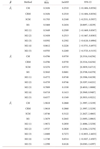
5. Real Data Analysis
In this section, we apply our proposed methods to analyze two datasets,
mu-shroom data and medical data, which are interval data corresponding to Model 1
or Model 2. The first data which we used to analyze is a mushroom data, which
is from the Fungi of California Species Index. The complete data can be
down-loaded from the internet site,
http://www.mykoweb.com/CAF/species_index.html
. Three features are represented
by three variables Y = the width of the pileus cap, X
1= the length of the stipe,
and X
2= the thickness of the stipe. These measurements in the dataset are
inter-val inter-value (in cm). There were 311 observations from the Fungi of California
Spe-cies Index. Because the lengths of the variables should depend on each other, the
dataset belongs to Model 1. By the method 1 and method 2 with the same
set-tings in simulations, we analyze the dataset and present the results in Table 9. In
Table 9, we present the estimations of
β
(
Beta
), the jackknife standard
devi-ation (JackSD) and the 95% confidence interval (95% CI). From the results in
Table 9, the M1 approach has smaller standard deviation in the estimations of
1
β
and
β
2. The SCM approach has smaller standard deviation in the
estima-tion of
β
0.
The next data which we used to analyze is a medical data, which is from
Bil-lard and Diday [6], and the dataset have 10,000 classical observations. Xu [4]
classified the entire data to form 42 categories by Agegroup × diabetes × race
(
7 3 2 42
× × =
). For the dataset, we consider three variables
Y = cholesterol
(chol), X
1= age, and X
2= income. The medical dataset should belong to Model 2,
because the lengths of the variables do not depend on each other. Then, apply
the method 1 and method 2 with the same settings in simulations to analyze the
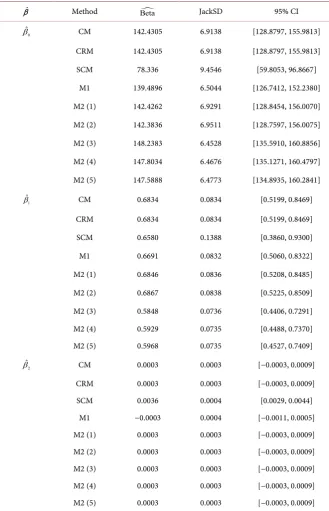
dataset and present it in Table 10. In Table 10, we present the estimations of
β
(
Beta
), the jackknife standard deviation (JackSD) and the 95% confidence
in-terval (95% CI). From the results, the inin-terval weighted LSE (M2) with W
3has
smaller standard deviation than others, which coincides with the results in
si-mulations. The age variable is significant and the income variable is not
signifi-cant. Furthermore, the average of cholesterol adds about 0.59 when age adds one
year.
6. Conclusion
impli-DOI: 10.4236/ojs.2018.86059 899 Open Journal of Statistics
cate the lengths of the interval data of the dependent variable and the
indepen-dent variables are correlated with each other. In some applications, the interval
lengths of the two variables may not depend on each other. Thus, for the
situa-tion, we consider model 2 data and suggest the interval weighted least squares
estimation method. In addition, we compare our proposed methods with CM
proposed by Billard and Diday [2], CRM proposed by Carvalho et al. [3] and SCM
proposed by Xu [4] via simulations. From simulation studies, the performance of
the endpoints LSE is similar to others for model 1 data. The interval weighted LSE
Table 9. Estimations of
β
for mushroom data.ˆ
β Method Beta JackSD 95% CI
0
ˆ
β CM 0.3436 0.2510 [−0.1484, 0.8356]
CRM 0.3436 0.2510 [−0.1484, 0.8356]
SCM 0.1703 0.2160 [−0.2531, 0.5937]
M1 0.5468 0.2434 [0.0697, 1.0239]
M2 (1) 0.3449 0.2509 [−0.1469, 0.8367]
M2 (2) 0.3458 0.2513 [−0.1467, 0.8383]
M2 (3) 0.0392 0.2302 [−0.4120, 0.4904]
M2 (4) 0.0612 0.2226 [−0.3751, 0.4975]
M2 (5) 0.0705 0.2260 [−0.3725, 0.5135]
1
ˆ
β CM 0.4786 0.0750 [0.3316, 0.6256]
CRM 0.4786 0.0750 [0.3316, 0.6256]
SCM 0.5276 0.0733 [0.3839, 0.6713]
M1 0.5043 0.0681 [0.3708, 0.6378]
M2 (1) 0.4772 0.0748 [0.3306, 0.6238]
M2 (2) 0.4759 0.0746 [0.3297, 0.6221]
M2 (3) 0.7009 0.1530 [0.4010, 1.0008]
M2 (4) 0.6718 0.1413 [0.3949, 0.9487]
M2 (5) 0.6577 0.1349 [0.3933, 0.9221]
2
ˆ
β CM 1.9618 0.2868 [1.3997, 2.5239]
CRM 1.9618 0.2868 [1.3997, 2.5239]
SCM 1.8746 0.3122 [1.2627, 2.4865]
M1 1.5679 0.2645 [1.0495, 2.0863]
M2 (1) 1.9672 0.2850 [1.4086, 2.5258]
M2 (2) 1.9727 0.2828 [1.4184, 2.5270]
M2 (3) 1.0400 0.7273 [−0.3855, 2.4655]
M2 (4) 1.1740 0.6514 [−0.1027, 2.4507]
DOI: 10.4236/ojs.2018.86059 900 Open Journal of Statistics
Table 10. Estimations of
β
for medical data (Y: chol, X1: age, X2: income).ˆ
β Method Beta JackSD 95% CI
0
ˆ
β CM 142.4305 6.9138 [128.8797, 155.9813]
CRM 142.4305 6.9138 [128.8797, 155.9813]
SCM 78.336 9.4546 [59.8053, 96.8667]
M1 139.4896 6.5044 [126.7412, 152.2380]
M2 (1) 142.4262 6.9291 [128.8454, 156.0070]
M2 (2) 142.3836 6.9511 [128.7597, 156.0075]
M2 (3) 148.2383 6.4528 [135.5910, 160.8856]
M2 (4) 147.8034 6.4676 [135.1271, 160.4797]
M2 (5) 147.5888 6.4773 [134.8935, 160.2841]
1
ˆ
β CM 0.6834 0.0834 [0.5199, 0.8469]
CRM 0.6834 0.0834 [0.5199, 0.8469]
SCM 0.6580 0.1388 [0.3860, 0.9300]
M1 0.6691 0.0832 [0.5060, 0.8322]
M2 (1) 0.6846 0.0836 [0.5208, 0.8485]
M2 (2) 0.6867 0.0838 [0.5225, 0.8509]
M2 (3) 0.5848 0.0736 [0.4406, 0.7291]
M2 (4) 0.5929 0.0735 [0.4488, 0.7370]
M2 (5) 0.5968 0.0735 [0.4527, 0.7409]
2
ˆ
β CM 0.0003 0.0003 [−0.0003, 0.0009]
CRM 0.0003 0.0003 [−0.0003, 0.0009]
SCM 0.0036 0.0004 [0.0029, 0.0044]
M1 −0.0003 0.0004 [−0.0011, 0.0005]
M2 (1) 0.0003 0.0003 [−0.0003, 0.0009]
M2 (2) 0.0003 0.0003 [−0.0003, 0.0009]
M2 (3) 0.0003 0.0003 [−0.0003, 0.0009]
M2 (4) 0.0003 0.0003 [−0.0003, 0.0009]
M2 (5) 0.0003 0.0003 [−0.0003, 0.0009]
with
W
3has better performance for model 2 data. Finally, we analyze two real
datasets for illustration. Furthermore, the results coincide with the results in
si-mulation studies.
Conflicts of Interest
DOI: 10.4236/ojs.2018.86059 901 Open Journal of Statistics
References
[1] Diday, E. (1987) Introduction à l’ Approache Symbolique en Analyse des Données.
Premières Journées Symbolique-Numérique. CEREMADE, Université Paris, 21-56.
[2] Billard, L. and Diday, E. (2000) Regression Analysis for Interval-Valued Data. In:Bock, H.-H. and Diday, E., Eds., Data Analysis, Classification and Related Methods, Springer-Verlag, Berlin, 369-374.https://doi.org/10.1007/978-3-642-59789-3_58 [3] Carvalho, F.A.T., Neto, L. and Tenorio, C.P. (2004) A New Method to Fit a Linear
Regression Model for Interval-Valued Data.
Annual Conference on Artificial
Intel-ligence: KI2004 Advances in Artical Inteligence,
Ulm, 20-24 September 2004, 295-306.https://doi.org/10.1007/978-3-540-30221-6_23[4] Xu, W. (2010) Symbolic Data Analysis: Interval-Valued Data Regression. Ph.D. Thesis, The University of Georgia, Athens.
[5] Billard, L. (2008) Sample Covariance Functions for Complex Quantitative Data. In: Mizuta, M. and Nakano, J., Eds.,