The “Ocean Stabilization Machine” May Represent a Primary Factor Underlying the Effect of “Global Warming on Climate Change”

(1)

ISSN Print: 2160-0414

DOI: 10.4236/acs.2019.91009 Jan. 10, 2019 135 Atmospheric and Climate Sciences

The “Ocean Stabilization Machine” May

Represent a Primary Factor Underlying the

Effect of “Global Warming on Climate Change”

Yanjun Mao

1

, Jiqing Tan

2*

, Bomin Chen

3

, Huiyi Fan

2

1_{Climate Center, Zhejiang Meteorologic Bureau, Hangzhou, China} 2_{Earth Science School, Zhejiang University, Hangzhou, China} 3_{Shanghai Climate Center, Shanghai, China}

Abstract

Contemporary references to global warming pertain to the dramatic increase in monthly global land surface temperature (GLST) anomalies since 1976. In this paper, we argue that recent global warming is primarily a result of natu-ral causes; we have established three steps that support this viewpoint. The first is to identify periodic functions that perfectly match all of the monthly anomaly data for GLST; the second is to identify monthly sea surface temper-ature (SST) anomalies that are located within different ocean basin domains and highly correlated with the monthly GLST anomalies; and the third is to determine whether the dramatically increasing (or dramatically decreasing) K-line diagram signals that coincide with GLST anomalies occurred in El Niño years (or La Niña years). We have identified 15,295 periodic functions that perfectly fit the monthly GLST anomalies from 1880 to 2013 and show that the monthly SST anomalies in six domains in different oceans are highly correlated with the monthly GLST anomalies. In addition, most of the annual dramatically increasing GLST anomalies occur in El Niño years; and most of the annual dramatically decreasing GLST anomalies occur in La Niña years. These findings indicate that the “ocean stabilization machine” might represent a primary factor underlying the effect of “global warming on climate change”.

Keywords

Global Warming, Monthly Global Land Surface Temperature (GLST) Anomalies, Monthly SST Anomalies, Ocean Stabilization Machine, K-Line Diagram Signals

How to cite this paper: Mao, Y.J., Tan, J.Q., Chen, B.M. and Fan, H.Y. (2019) The “Ocean Stabilization Machine” May Represent a Primary Factor Underlying the Effect of “Global Warming on Climate Change”. Atmospheric and Climate Sciences, 9, 135-145. https://doi.org/10.4236/acs.2019.91009 Received: December 10, 2018 Accepted: January 7, 2019 Published: January 10, 2019

http://creativecommons.org/licenses/by/4.0/

(2)

DOI: 10.4236/acs.2019.91009 136 Atmospheric and Climate Sciences

1. Introduction

Global climate changes are controlled by major periodic factors that represent basic principles in climatology, such as solar radiation, atmospheric circulation and oceans. A number of scientists subjectively consider that the recent dramatic upward trends in monthly GLST anomalies represent non-periodic and irre-versible changes and postulate that warming related to the global greenhouse ef-fect has primarily been caused by anthropogenic emissions. However, with the decline of global warming, an increasing number of scientists have started to question this view [1]-[12]. There are two primary methods challenging the hy-pothesis that recent global warming is caused by anthropogenic emissions: the first method is to prove that the recent dramatic upward trend of monthly GLST anomalies is periodic, and the second method is to link global warming to major factors in nature. In our opinion, the oceans on this planet can be vividly called “ocean stabilization machines” (OSM). When some parts of an OSM lose control for unknown reasons, other parts of the OSM function stabilize the atmospheric circulation. As a result, El Niño or La Niña events occur. According to this viewpoint, in the historical data of the monthly SST anomalies, we would find out some significant information. Therefore, we work out a research plan to confirm our viewpoint. We first developed a numerical functional analysis me-thod to identify periodic functions that perfectly fit the monthly GLST anoma-lies from 1880 to 2013. This study can make us clearly to understand the nature of the dramatic rises signals of monthly GLST anomalies. Second, we defined El Niño and La Niña years based on the K-line diagram technique [13] because the ENSO phenomenon is the strongest year-to-year climate fluctuation on our pla-net and produces worldwide impacts to both natural systems and human socie-ties [14] [15]. Third, we calculated the correlation coefficients between the monthly GLST anomalies and the monthly gridded sea surface temperature (SST) data anomalies obtained from the Hadley Centre for the period 1880 to 2007. This study can help us to know whether there were some dramatic rises signals existed in the historical data of the monthly SST anomalies. This information would help us to link the monthly GLST anomalies with oceans. Fourth, we have analyzed the monthly GLST anomaly data using the K-line diagram technique to determine if the annual dramatic upward (or downward) monthly GLST ano-maly signals are highly associated with El Niño and La Niña years.

2. Data and Methods

2.1. Data

In this paper, we use two sources of data: the first is SST data from Hadley cli-mate center; the second is the monthly global land surface temperature (GLST) anomaly index data downloaded from the official website of NOAA.

2.2. Methods

2.2.1. The Numerical Functional Analysis Technique (NFAT)

(3)

DOI: 10.4236/acs.2019.91009 137 Atmospheric and Climate Sciences the following formula (1):

( )

(

)

1 sin , 1,2, ,

N i

i i

F t a t c i N

b π

=

∑

+ = _ ₍₁₎

where ai, bi and c are constant coefficients and t is time. The function t is

calculated with following formula:

(

1879

)

12

n

t= m− +

where m is the numerical year and n is the numerical month, e.g.,

1,2, ,12

n=  .

In NFAT, ai, bi, and c are variables that increase at the interval of 0.001 to

search the best values and automatically calculating the correlated coefficients and root mean square between the function values and the historical monthly global land surface temperature (GLST) anomaly index data with a computer on the platform of Linux software system.

2.2.2. The K-Line Diagram Technique

The K-line diagram technique was developed in the 18th century and is widely used in the stock market to avoid random noise. This method provides a tool that investors can use to extract signals that occur before a sudden change in the price of a stock. Based on the extracted signals, investors purchase a stock at a low price and the sell stock at a high price, thereby earning a large amount of money. In the K-line technique, K-line diagrams are drawn using four-dimensional data ac-cording to the opening price, the maximum price, the minimum price and the closing period price. The diagrams are categorized into three types: Yang lines, Yin lines and crossed lines.

1) Using K-line diagram technique to draw annual GLST anomaly K-line dia-gram

A map of the K-line figures drawn using the monthly data to draw annual K-line diagram is called an annual K-line diagram. In mathematics, the four-dimensional data is needed to draw an annual K-line diagram. In this study, we define the four-dimensional composite data as follows.

The first dimension of the data is the monthly GLST anomalies in January; the second dimension is the monthly maximum GLST anomaly in a year; the third dimension is the monthly minimum GLST anomaly in a year; and the fourth dimension is the monthly GLST anomaly in December.

2) Different types of K-line diagrams

The K-line diagrams show the different types of variations in GLSTs using different figures. In general, there are three categories of K-line diagrams: Yang line diagrams, crossed line diagrams and Yin line diagrams.

To provide more specific information for readers, we have presented several examples to introduce the different types of K-line diagram signals.

(4)

[image:4.595.210.536.69.286.2]

Figure 1. Ten kinds of K-line diagrams.

a) Long solid Yang line (A of Figure 1)

If the monthly SST anomalies within a year are estimated as follows: Jan, Feb, Mar, Apr, May, Jun, Jul, Aug, Sept, Oct, Nov, Dec

−0.49, 0.3, −0.2, 0.2, 0.3, 0.1, 0.2, 0.3, 0.1, 0.3, 0.4, 0.49

the K-line diagram technique renders the information for this year as a long sol-id Yang line signal.

b) Long solid Yin line (B of Figure 1)

0.49, 0.4, 0.3, 0.1, 0.3, 0.2, 0.1, 0.3, 0.2, −0.2, −0.3, −0.49,

the K-line diagram technique renders this information as a long solid Yin line. c) Long Yang line body below a shadow line (C of Figure 1)

−0.49, −0.3, −0.2, 0.2, 0.3, 0.8, 0.2, 0.3, 0.1, 0.3, 0.4, 0.49

the K-line diagram technique renders this information as a strong upward sig-nal; however, the position of the shadow line indicates a degree of resistance that is preventing the signal from increasing.

d) Long Yang line body above-mentioned shadow line (D of Figure 1) If the monthly SST anomalies within a year are estimated as follows: Jan, Feb, Mar, Apr, May, Jun, Jul, Aug, Sept, Oct, Nov Dec

−0.49, −0.3, −0.2, 0.2, 0.3, −0.6, 0.2, 0.3, 0.1, 0.3, 0.4, 0.49

the K-line diagram technique renders this information as a strong upward signal with a supporting signal in June, and the position of the shadow line indicates that there is an upward force that is increasing the signal.

(5)

DOI: 10.4236/acs.2019.91009 139 Atmospheric and Climate Sciences Jan, Feb, Mar, Apr, May, Jun, Jul, Aug, Sept, Oct, Nov, Dec,

−0.49, −0.3, −0.2, 0.2, 0.3, −0.6, 0.2, 0.3, 0.8, 0.3, 0.4, 0.49

the K-line diagram technique renders this information as a strong upward signal with an upward force in June and a resistance force in September; in addition, because the length the shadow line above is longer than the shadow line below, the resistance force is greater than the upward force.

The Long Yin line body below a shadow line (F of Figure 1), the Long Yin line body above a shadow line (G of Figure 1), and the Long Yin line body with both shadow lines (H of Figure 1) have similar meanings to that of the Yang body, and the only difference is that the direction of the main body is reversed.

The meanings of the Long Yang cross line (I of Figure 1) and the long Yin cross line (J of Figure 1) are similar, which suggests that the main signal is dri-ven by two opposing factors.

3. Results

3.1. The Study on If the Dramatic Signals of GLST to Be Periodical

or Not

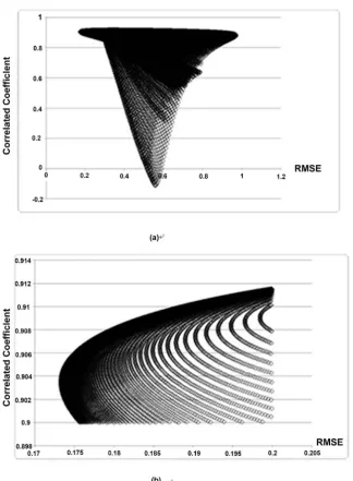
Figure 2(a) illustrates the verification results of 173,000 periodic functions iden-tified during the final search of the NFAT system; the x axis displays the root mean square error between the values of functions and the monthly global land surface temperature (GLST) anomaly index data from 1880 to 2013, and the y axis displays the correlation coefficients between the values of functions and the monthly global land surface temperature (GLST) anomaly index data from 1880 to 2013. Figure 2(b) shows the verification results of 15,295 distinct periodic functions from a total of 173,000 periodic functions. The verification results of the 15,295 distinct functions are provided in Figure 2(a); the coefficients are all greater than 0.9, and the RMSE values are all less than 0.2.

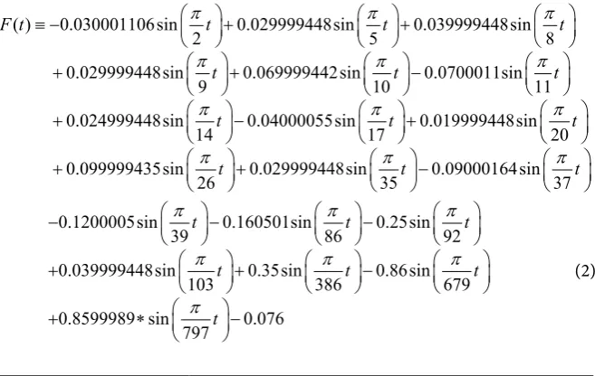
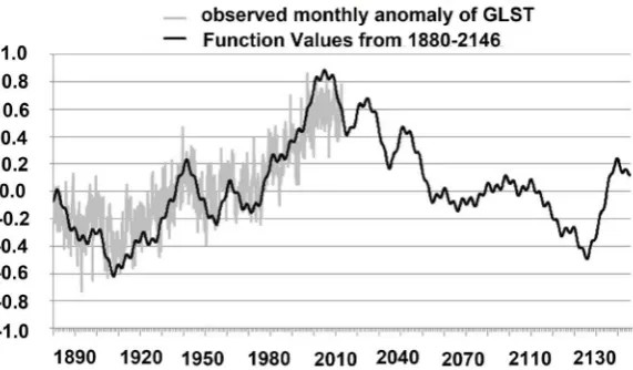
Figure 3 illustrates values of the best function (see formula 2) and the ob-served monthly GLST anomalies from 1880 to 2013 and shows the calculated results from 2014 to 2146.

( ) 0.030001106sin 0.029999448sin 0.039999448sin

2 5 8

0.029999448sin 0.069999442sin 0.0700011sin

9 10 11

0.024999448sin 0.0 14

F t t t t

t t t

t

π π π

π       ≡ − _ _+ _ _+ _ _             + _ _+ _ _− _ _         + _ _−

  4000055sin 17 0.019999448sin 20 0.099999435sin 0.029999448sin 0.09000164sin

26 35 37

t t

t t t

π π

π π π

 ₊                 + _ _+ _ _− _ _      

0.1200005sin 0.160501sin 0.25sin

39 86 92

0.039999448sin 0.35sin 0.86sin

103 386 679

0.8599989 sin 0.076

797

t t t

t

π π π

[image:5.595.209.538.530.738.2]

(6)

[image:6.595.212.537.64.506.2]

Figure 2. The verification results for 173,000 periodic functions and 15,295 special peri-odic functions. Note: (a) Verification results of 173,000 periperi-odic functions during the fi-nal searching in NFAT system. Note that the x axis is the root of mean square error which is one of the verification quantities to check the simulated effect in numerical simulation study; y axis is the correlated coefficient which is also another quantity to check if two time series data match each other. (b) Verification results of 15,295 special functions in (a), which their coefficients are all greater than 0.9, and RMSE are all less than 0.2.

(7)

[image:7.595.230.516.72.239.2]

Figure 3. The anomaly of global land surface temperature (1880-2013) and the fitting function value from 1880 to 2146.

the lowest point in November, 2127, which is −0.49456˚C. According to the er-ror in previous time, for example, it reached the lowest point in January, 1908, which was minus 0.61946˚C (in fact, it was in October, 1892, when the anomaly is −0.73˚C). The prediction using the function had 16 years lag, and −0.11054˚C underestimated. Thus, we amend our prediction as it will reach −0.6051˚C in 2111.

3.2. The Study on Linking the Dramatic Signals of GLST with SST

Anomalies

Figure 4 illustrates the geographic distribution of the correlation coefficients between the GLST monthly anomalies and SST anomalies at all grid-points worldwide. We can see that the monthly anomaly of SST in six domains of oceans are highly correlated with the monthly anomaly of GLST: five domains marked as A, B, C, D and E are found to be high positively correlated with GLST; one domain marked as F is found negatively correlated with the monthly anomaly of GLST. In this figure, we have also marked the four box domains where SST data is used by climatologists to calculate NINO 1+2, NINO 3, NINO 3.4 and NINO 4 indices. In our opinion, if we desire to define the index for gauging El Niño (or La Niña) events, the NINO index should be in B domain where correlated coef-ficient is higher. Besides, to link the SST anomalies with ocean stabilization ma-chine, the other domain such as A, C, D, E and F should be paid much more at-tentions.

3.3. The Study on Monthly Dramatic Upward and Downward

Signals between GLST Anomalies and SST Anomalies

(8)

[image:8.595.211.533.76.397.2]

Figure 4. The geographical correlated-coefficient fields between monthly SST anomalies and monthly global land surface temperature anomalies and four square areas for calcu-lating NINO 1+2, NINO 3, NINO 3.4 and NINO 4.

(9)

[image:9.595.213.536.72.284.2]

Figure 5. Annual K-line diagrams of global land surface temperature (1950-2012).

downward at low positions at the end of the year, and the k-line diagram was at lower position than that in previous year.

These results provided us with evidences which observed monthly GLST anomalies from 1950 to 2012 is highly correlated with ENSO, which support our viewpoint of ocean stabilization machine (OSM) [13].

4. Discussion

In science, when there are two or more ideas to be employed to explain the re-cent global warming, we always trust which can fit perfectly all the observed monthly anomaly of GLST from 1880 to now. Until now, no one claims that he can fit perfectly the observed monthly anomaly of GLST from 1880 to now as we do. We have found 15,295 periodic functions with NFAT, which their coeffi-cients are all greater than 0.9, and RMSE are all less than 0.2; therefore, we have proved that the recent dramatic upward trend of GLST can still be periodic changes. The function with best verification result has also been employed to predict the future behavior of the monthly anomaly of GLST; we can see that the downward trend for the monthly anomaly of GLST had already begun; it will reach the lowest point at −0.6051˚C in 2111.

(10)

DOI: 10.4236/acs.2019.91009 144 Atmospheric and Climate Sciences study. Furthermore, we noticed that the four domains to measure Nino 1+2, Nino 3, Nino 4 and Nino 3.4 are located at some latitude belts which the corre-lated coefficients between the monthly anomaly of GLST and the monthly ano-maly of SST are about 0.2. In our opinion, if the NINO indices are defined in-cluding the B domain, it would better to link El Niño (or La Niña) events with global climate changes. Using the new terms of “El Niño years, La Niña years and normal years” based on the ocean stabilization machines (OSMs) viewpoint [13], we can find some very interesting phenomena: most dramatic upward k-line diagram signals occurred in El Niño years; most crashing downward k-line diagram signals occurred in La Niña years. These findings have effectively supported the OSM viewpoint: the oceans on this planet can be vividly called “ocean stabilization machines” (OSM). When some part of an OSM loses control for unknown reasons, other parts of the OSM stabilize the atmospheric circula-tion. As a result, El Niño or La Niña events occur.

5. Summary

In this paper, we have found that the dramatic upward rising signals can be per-fectly fitted with periodic functions, which suggests that the major climate fac-tors can still be the main reason for the recent global climate warming, and the secondary climate factor such as anthropogenic emissions might be the second-ary reason. If we use the best function to predict the future behaviour of GLST, we can know that the downward trend for the monthly anomaly of GLST had already begun, and it will reach −0.6051˚C in 2111. The correlation study tells us that the dramatic anomalies can be seen in SST fields of different oceans, which might be the results of OSM, and with the k-line diagram technique, we can see that most of the annual dramatically increasing GLST anomalies occur in El Niño years; and most of the annual dramatically decreasing GLST anomalies occur in La Niña years. These findings show us how OSM works. In a word, al-though there are many academic topics need to study further in future, we can still make a conclusion: “OSM” might play a very important role to cause global climate changes.

Acknowledgements

This paper is supported by three projects: one is by National Natural Science Foundation of China (Grant NO. 40875091), two is by Special Scientific Re-search Project for Public Interest (Grant NO. GYHY201306021), and three is the National Key Research and Development Program of China “major natural dis-aster monitoring warning and prevention” (Grant No. 2017YFC1502301), the authors has no competing interests.

Conflicts of Interest

(11)

References

[1] Chen, X. and Tung, K.-K. (2014) Varying Planetary Heat Sink Led to Glob-al-Warming Slowdown and Acceleration. Science,345, 897-903.

https://doi.org/10.1126/science.1254937

[2] Easterling, D.R. and Wehner, M.F. (2009) Is the Climate Warming or Cooling?

Geophysical Research Letters,36, Article ID: L08706.

https://doi.org/10.1029/2009GL037810

[3] Fyfe, J.C., Gillett, N.P. and Zwiers, F.W. (2013) Overestimated Global Warming over the Past 20 Years. Nature Climate Change,3, 767-769.

https://doi.org/10.1038/nclimate1972

[4] Meehl, G.A., Arblaster, J.M., Fasullo, J.T., Hu, A. and Trenberth, K.E. (2011) Mod-el-Based Evidence of Deep-Ocean Heat Uptake during Surface-Temperature Hiatus Periods. Nature Climate Change,1, 360-364. https://doi.org/10.1038/nclimate1229

[5] Risbey, J.S., et al. (2014) Well-Estimated Global Surface Warming in Climate Pro-jections Selected for ENSO Phase. Nature Climate Change, 4, 835-840.

[6] Curry, J.A. and Webster, P.J. (2011) Climate Science and the Uncertainty Monster.

Bureau of the American Meteorological Society,175, 1667-1682.

https://doi.org/10.1175/2011BAMS3139.1

[7] Loehle, C. (2007) A 2000 Year Global Temperature Reconstruction Based on Non-Tree Ring Proxies. Energy & Environment,18, 1049-1058.

https://doi.org/10.1260/095830507782616797

[8] Lindzen, R.S. (2007) Taking Greenhouse Warming Seriously. Energy & Environ-ment, 18, 937-948. https://doi.org/10.1260/095830507782616823

[9] Holland, M. (2013) The Great Sea-Ice Dwindle. Nature Geoscience, 6, 10-11.

https://doi.org/10.1038/ngeo1681

[10] Seneviratne, S., et al. (2014) No Pause in the Increase of Hot Temperature Extremes.

Nature Climate Change,4, 161-163. https://doi.org/10.1038/nclimate2145

[11] Kosaka, Y. and Xie, S.-P. (2013) Recent Global-Warming Hiatus Tied to Equatorial Pacific Surface Cooling. Nature,501, 402-407. https://doi.org/10.1038/nature12534

[12] England, M., et al. (2014) Recent Intensification of Wind-Driven Circulation in the Pacific and the Ongoing Warming Hiatus. Nature Climate Change,4, 222-227.

[13] Tan, J. (2015) A Most-Recognized Principle to Define El Niño and La Niña Years Based on the K-Line Diagram Technique. International Journal of Climatology, 35, 2777-2782. https://doi.org/10.1002/joc.4171

[14] McCreary, J., Zebiak, S.E. and Glantz, M.H. (2006) ENSO as an Integrating Concept in Earth Science. Science, 314, 1740-1745. https://doi.org/10.1126/science.1132588

[15] Mcphaden, M.J., Timmermann, A., Widlansky, M.J., Balmaseda, M.A. and Stock-dale, T.N. (2015) The Curious Case of the EL NIÑO That Never Happened. Bulletin of the American Meteorological Society, 96, 1647-1665.