A New Method of Construction of Robust Second Order Rotatable Designs Using Balanced Incomplete Block Designs

A New Method of Construction of Robust Second Order

Rotatable Designs Using Balanced Incomplete Block

Designs

Bejjam Re. Victorbabu, Kottapalli Rajyalakshmi

Department of Statistics, Acharya Nagarjuna University, Guntur, India Email: [email protected]

Received December 8,2011; revised December 30, 2011; accepted January 12, 2012

ABSTRACT

Das [1,2] studied robust second order rotatable designs (RSORD) and constructed second order rotatable designs with correlated errors (SORDWCE) under the auto correlated structure using central composite design. In this paper, a new method of construction of RSORD using balanced incomplete block designs (BIBD) is suggested. In this method the number of design points required is in some cases less than the number required in Das [1,2] method of construction of robust rotatable central composite designs (RRCCD). We may point out here that this RSORD using BIBD has 113 design points for 7-factors where as the corresponding RRCCD obtained by Rajyalakshmi and Victorbabu [3] needs 157 design points. Thus the new method leads to a 7-factor RSORD in less number of design points than the corre-sponding RRCCD. Here we also obtained the variance of the estimated response for the factors 3 ≤v≤ 8.

Keywords: Response Surface Designs; Rotatability; Second Order Rotatable Designs (SORD); Robust SORD;

Robustness; Balanced Incomplete Block Designs

1. Introduction

In response surface methodology, rotatability is a natural and highly desirable property. This was introduced and developed by Box and Hunter [4], assuming the errors to be uncorrelated and homoscedastic. Das and Narasim- ham [5], constructed second order rotatable designs (SORD) through balanced incomplete block designs (BIBD). Pan- da and Das [6] studied first order rotatable designs with correlated errors. Further, Rajyalakshmi and Victorbabu [3] extended the work of Das [1,2] and constructed RRCCD for 3 ≤v≤ 17.

In order to study the nature of robust rotatable designs, rotatability conditions for second order regression de- signs have been derived, assuming the errors to be corre- lated. These conditions have been further studied under different variance covariance structures of errors. Here we derive conditions for rotatability for a general corre- lated errors structure and specialize then to the auto- correlated structure.

In this paper, a new method of construction of RSORD using BIBD is suggested and also obtained the variance of the estimated response for factors 3 ≤v≤ 8.

2. Conditions of SORDWCE

Assuming that the response surface is of second order, we adopt the model:

1 0

1

v v

u i iu ij iu ju u

i

i j

y   x  x x e

  

 





 



2 0

1 1 1

ˆ ˆ v ˆ v ˆ v ˆ

(1) where Y is the vector of recorded observations on the study variable y,β’s are the vector of regression coeffi-cients, euare random errors with correlated errors.

2.1. Conditions of Rotatability The estimated response at x is given by

x ii i i i ij i j

i i i j

x x x x

y    

   

 









 

ˆ

(2) The variance of estimated response at yx

 



is given by



 





 

















 

4 2 2 2 2

0 0 0

1 1 1 1 1

3 2 2 2

1 1 1 1

ˆ ˆ _{2 ( ,}ˆ ˆ _{) 2} ˆ _,ˆ ˆ ₂ ˆ ˆ_,

ˆ ˆ ˆ ˆ ˆ ˆ ˆ

2 , 2 , , 2

ˆ

2

v v v v v

x i ii i ii i j ii jj i i i i

i i i j i i

v v v v

i j i j i i ii i j ii j i j ij

i j i i j i j

V V x V x Cov x x Cov x V x Cov

x x Cov x Cov x x C v x x V

y

o

        

      

     

      

     

    





 





 



 

 















   





0 1

2

1 1 1 1 1 , ,

ˆ ˆ_,

ˆ ˆ ˆ ˆ ˆ ˆ

2 , 2 , 2 ,

v

i j ij

i j v

s i j ss ij s i j s ij i j l t ij lt

s i j s i j i j l t i j l t

x x Cov

x x x Cov x x x Cov x x x x Cov

 

     

 

         



 

 



















0. 1 2 . 1 v i i v ii j i j i j x v

x x v    



. . 1 1 v

 

00 4 . 2 0.

1 1

2 2 . 2 .

1 1

. 3 .

1 1

2 2 . 0.

1 1 2 1 1 2 2 2 2 2 2 2 ˆ 2 v v

ii ii ii

x i i

i i

v v

ii jj i i

i j i

i j i i

v v

i j i ii

i j i

i j i

v v

ij ij ij

i j i j

i j i j

v

s i j

s i j

V v x v x v

x x v x v

x x v x v

x x v x

x y x v x x                          





 





 





 

 

  

    . 1 , ,

2 2 ss ij s i v ij lt

i j l t

i j l t i j l t

x x x x v        

  

   

s ij

s i j

j

v x x x v



(4) The variance function in (3) will b tion of 2

1

v

i i e a func x





for rotatab_{ility for all x if v}0.i_v0.ij _vi.j _{0; 1 ≤i≠j≤}

v; _vii j. _{0; 1≤i, j≤ v; v}s ij. _vss ij. _{0; 1 ≤ s, i < j≤ v;}

. ₀

ij lt

v  ; 1 0.ii _constant

1 a

 , say; 1≤ i ≤ v;

.ij _constant ≤i, l < j, t≤v, (i, j)

≤ i ≤ v; _vi i. _{= const}

1

tant

v  d , say; 1 ≤ i

≤i < j≤v; and

≠ (l, t); v ant = e

≠ j ≤ v; _vij

, say; 1

cons

, say; 1

.

ii jj

c

 ii ii.

1

2

c v constant d ; 1

≤

ability designs with corre

del (1 elements of th

.

i j

(iii) (1) v 0 .

i jl < l≤v

≤i v.

Below are given equivalent conditions for rotat in second order regression lated errors mo ) in terms of the e moment matrix:

0.j 0.jl 0

v v  ; 1 ≤j < l ≤v ii) v 0; 1 ≤i≠j ≤v

; 1 ≤i, j≤v (I): (i)

(

.

ii j

(2) v 0; 1 ≤i, j (3) vii jl.. 0; 1 ≤i, j < l≤v

(4) vij lt_. 0; 1 ≤i, l< j, t≤v, (i, j) ≠ (l, t) (II): (i) v_0.jj constanta₀, say; 1 ≤j≤v

(ii) vi i. constant _e, sa 1

  y; 1 ≤i≤v

(iii) v_ii.iiconstant  2 f c

 

  

 , say; 1 ≤i≤v (III): (i) vii.jj constant f ; 1 ≤i≠j≤v

(ii) . ta

1 nt ij

v cons  ; 1 ≤i < j≤v c



.  ij ij. vii jj. ; 1 ≤i < j≤ v (5) e Function of SORDWCE

The estimated response at x is given by

2 0

1 1 1

ˆ ˆ ˆ ˆ

ˆ v v v

ij

(IV): v_{ii ii} 2v 2.2. Varianc

x i i ii i ij i j

i i i j

x x

y     x x

   

 









 

(6)

The variance function of a SORDWCE is given by

 

 

 





 

 





2 0 0 1

4 2 2

1 1

2 2 2

1 1

00

1 1

ˆ _{2 ( ,}ˆ ˆ ₎

ˆ ₂ ˆ _, ˆ

ˆ ˆ

2

ˆ_x v _{i ii}

i

v v

i ii i j ii jj

i i j

v v

i i i

i i j

V V x Cov

x V x x Cov

x V x x V

v d

y

a e d

  



2 4

2 (c d )

j ij                    





 



 

(7) 2 1

whi a function of i d





When the erro

reduce respectively to the usual second order rotatability iance

func-2.3. Conditions for Exact Rotatability Following (4), necessary and sufficient conditio se

it is si

   

0. 1

1 2

I * i j N ju N ju 0, 1 ;

u u

v x  x j v

 









  

1 0.

1 2

0, 1 ;

N N

jl ju lu ju lu

u u

v x x  x x j l v

 

 

2

ch is



vxi

Note: rs are homoscedastic, (5) and (7)

conditions, non-singularity condition and var tion.

ns for cond order rotatability under auto-correlated structure,

mplifies to 

_



_

   

 

    1 2 . 1 2 1 1 1 1 1 1 ii

0, 1 ;

N N

i j iu ju iu ju

u u

N N

iu j u i u ju

u u

v x x x x

x x x x i j v

                _  _     









 1  1 1 iu j u 1 i u ju

u u

  

2 2 1 2

.

1 2

1 1

2 2

iii 1

0, 1 , ;

N N

ii j iu ju iu ju

u u

N N

v x x x x

x x x x i j v

                _  _  









 

 1  1  1

1 , ;

ju l u i u j u lu

i j l v

  

 

_{2 v } N_{x x x }2N1_{x x x} .

1 2

1 1

1 1

0,

ij l iu ju lu iu ju lu

u u

N N

iu

u u

x x x x x x

          _   









    

 

    1

2 2 2

. 1 2 1 1 2 2 ( 1) 1 1 1 1 3 0, 1 , N N

ii jl iu ju lu iu ju lu

u u

N N

iu j u l u i u ju lu

u u

v x x x x x x

x x x x x x

 

      1 2 . 1 2 1 1

1 1 1

1 1

4

1 , ,

N N

ij lt iu ju lu tu iu ju lu

u u

N N

iu ju l u t u i u j u

u u

v x x x x x x x

x x x x x x

i l j t

                 









 1 0,

tu lu tu x x x   _     1 2 2 1 2 N N

   



₂



₂





1





0.

0

II * i 1 1

;1 ;

jj ju ju

u u x      _    





   v x

a j v

         

 









. 1

2 2 2 2 2

1 1

1 1

1 1

1 2

1_{,1 ;}

i i

N N N

iu iu iu i u

u u u

x x x x

i v e        _                







 

  ii v









. 1 1 2 2 1 1 iii 2 ii ii N

iu i u u v x x       _   



 1

2 2 4 2 4

1 2

1

2 _{, 1 ;}

N N

iu iu

u u

x x

d i v

c         _    _  _    





   









  1 2 2 1 1

2 2 2 2 2 2 2

1 2 1

1

(

, 1 ;

N N N

iu ju iu ju iu j u

u u u  

.

1

2 2

1 1

1 III * i ii jj

N

ju i u u

v

x x x x x x

d i j v

             _{ } 

 _ x _ x

   _     







 





   









. 1

ii vij ij



2 2

1 1

2 2 2 2 2

1 1

1 2 1

1

2

1_{, 1 ;}

N N N

iu ju iu ju iu ju i u j u

u u u

x x x x x x x x

i j v c       _{ }        _   _      







 

IV *vii ii. 2vij ij. vii jj. ,1  i j v; (8)

are as in (II)*(iii) and (III)*(i), ularity is given by,

(V)* :

where vii ii. ,vii jj. andvij ij. (ii).

The condition for non-sing 2 0 00

2 a ₀

v f

c v

 

   

  (9)













where _{N 2} 2 ₁

00

v  N     and 0 1_{, ,f a} c are as in (6).

ility, as stipu-nce ρ is

un-known unless special efforts are made regarding choice of the underlying robust design. Towards this, tremen-dous simplification obtains whenever all odd moments of various types vanish. These are listed below for ready re ference,

1 1

1 2 1 2

, ,1 ; , ,

N N N N

Note: The conditions fo lated above, are hard to satis

r exact rotatab fy in practice si

-

ju ju iu ju iu ju

u u u u

x x j v x x x x

     

 





    1 1 1 1 1 1

, ,1 ;

N N

iu j u i u ju

u u

x x x x i j v

        





  1 1

2 2 2

1

1 2 1

, , ,

N N N

iu ju iu ju iu j u

u u u

x x x x x x _

  







  1 2 1 1 1

;1 , ; ,

N N

ju iu ju lu

i u

u u

x x i j v x x x

 

 

 





1 1 1

, , ,

, ;

N N N

ju lu iu ju l

u  1  1  1

2 1 1

1

iu u i u j u lu

u u

x x x x x x x x x

i j l v

  









2 2 2

2 1

, iu ju lu, iu

u u u

x x x x x x x x x









 

1 2

1 ,1 , ;

N ju lu i u        

 1 ( 1)

1 iu ju lu j u l u

 

1 1

N N N

x

1

u

x x i j l v

     



1 , ,

1 tu 2 iu ju lu tu

u u

N N

iu ju lu x x x x





x x x x

      1 1 1 1 , N

iu ju l u t u u

x x x x

   



    1 1 1 1

;1 , , . N

lu tu i u j u u

x x x x i l j t v



 



  



(10) As to the even order moments (up to order 4) mere constancy of such moments (of various ty s) suffices to ensure exact rotatability. Specially, we sire to have each of the following terms independent of i and j:

2 2 1 ,1 ; N iu u pe de

x constant N v

 i    



4 4 1

3 ,1 ;

N

iu u

x constant N i v

    



2 2 4 1 ,1 ; N iu ju u

x x constant N i j v



    



Using the above relations, for the newly nstructed design, we get the following:

1 2 2 1 ,1 N iu u co

x constant N i v     



1 4 4 1

3 ,1 ;

N

iu u

x constant N i v 

   

2 2

4 1

N

iu ju u

,1 x x constant N



 



  i j v (11)

Thus, a design satisfying the conditions mentioned above may be successfully uti table design under violation of the homoscedasticity assumption sub-ject to the covariance structure being of the type (condi-tions of exact rotatability). Such a design is, therefore, robust, N, N1, ₄

lized as a rota

where c,  ,₂ are constants.

3. New Method of Construction of RSORD

ts by incorporating (n + 1) central points in the foll wing way.

One central point is placed in between each pair of non- central design points in the sequence, resulting thereby in (n – 1) such central points. The other two central points are placed one at the beginning and one at the end.

If the number of central points of the usual SORD with which we started is greater than (n + 1), the remaining central points are placed in any manner, if the number is le

examine the non-singularity for the original design and the newly constructed design.

Let N be the number of design points of he original design (SORD) with which we started. Out of N, let n be the number of non-central design points an m be the number of central points i.e., N = n + m. In general m < n + 1, Let N1 be the number of design points of the newly constructed design, Where N1 = 2n + 1 > N.

original design with which we started, the follo th

Using Balanced Incomplete Block Design

Here we start with usual SORD using BIBD having “n” non-central design points involving v-factors. The set of n design points can be extended to (2n + 1) poin

o

ss, we need to include the requisite number of addi- tional central points. Here we

t d

For the wing are e moment relations:

Let (v, b, r, k, λ) denote a BIBD. 2t k _{denote a}

frac-tional replicate of 2k _{in ±1 levels, in which no interaction}

with less than five factors is confounded and m be the number of central points in the design.

The design points for the newly constructed design are obtained as follows:

3.1. Method I: When r < 3λ

( )

t k

Here, N b 2    2v m n m and N1 = 2n + 1, where ( )

2t k 2 n b  v.

From the design points generated from the BIBD, simple symmetry conditions (10) and (11) are true. Con-ditions (10) are true obviously. ConCon-ditions (11) are true as follows:

 

2 2

2 1

2 2 ,

N

t k iu u

x r  N



  



 

4 4

4

2 2 3 ,

N

t k iu

x r N

1

u

 

  



 

2 2

4 1

2 ,

N

t k iu ju u

x x N



 



 



Using the above relations, for the newly constructed design, we get the following:

 

1

2 2

2 1

2 2 ,

N

t k iu u

x r  N



  



 

1

4 4

4 1

2 2 3 ,

N

t k iu u

x r  N



  



1 2 2

N

  t k

4 1

2

iu ju

u

x x  N



  (12) The results are given in Table 1.

3.2. Method II: When r = 3λ



Here, _{N b2}t k( )_m ( )

t k = n + m and N1 =2n + 1, where n=

2 b .

ted from the BIBD sim-metry conditions (10) a

0) are t obviously. C fo

From the design points genera

ple sym nd (11) are true. Condi-tions (1 rue onditions (11) are true as

llows:

 

2

2 1

2 ,

N

t k iu u

x r N



 



 

4

4 1

2 3 ,

N

t k iu u

x r N



 



 

2 2

4 1

2 ,

N

t k iu ju u

x x  N



 



Using the above relations, for the newly constructed design, we get the following:

 

1 2

N

t k

2 1

2 ,

iu u

x r N



 



1

N

  4

4 1

2t k 3 ,

iu u

x r N



 



 

1 2 2

4 1

2

N

t k

iu ju

u

x x  N



 



(13) The results are given in Table 2.

3.3. Method III: When r > 3λ Here, _{N b2}t k( )_2t v( )_{m = n +}

( ) ( )

t k t v m and N1 = 2n + 1,

Where n = 2b 2

ed from the BIBD sim-metry condit

0) are true ob fo

From the design points generat

ple sym ions (10) and (11) are true. Condi-tions (1 viously. Conditions (11) are true as

llows:

 

2 ( ) 2

2 1

2 2 ,

N

t k t v iu

u

x r  N



  

[image:5.595.54.547.101.736.2]

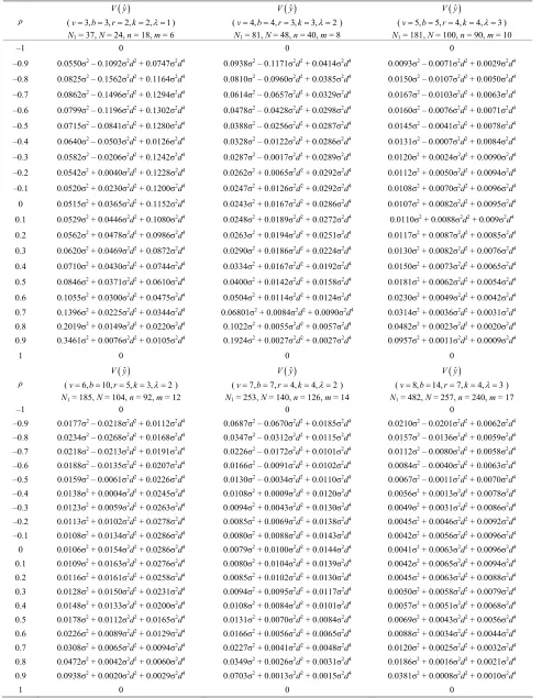
Table 1. Variance of the estimated response for the factors3 ≤v ≤8, when r < 3λ.

 ˆ

V y

2, 2, 1

r k

 ˆ

V y

,r

(v 4,b 4

ρ (v3,b3, 

N1 = 37, N

 

= 24, n = 18, m = 6

 )   3,k 3, 2

N1 = 81, N



= 48,

 ˆ

V y

,r 4,k 4, 3

  )

n = 40, m = 8

(v5,b5

N = 100,



   )

n = 90, m = 10

1 = 181, N

–1 0  0  0 

–0.9 0.0550σ2 _{– 0.1092σ}2_d2 _{+ 0.0747σ}2_d4 _0.0938σ2 _{– 0.117 4σd 0.0093} 2 2 2 4

–0.8 0.0825σ2 _{– 0.1562σ}2_d2 _{+ 0.1164σ}2_d4 _0.0810σ2 _{– 0.0 5σ}2_d4 _.0

–0.7 0.0862σ2 _{– 0.1496σ}2_d2 _{+ 0.1294σ}2_{d σ}2 _{– 0.065}

0.0

+ 0.1280σd  0.0388σ – 0.0

–0.4 0.0640σ2 _{– 0.0503σ}2_d2 _{+ 0.0126σ}2_d4

  0.0328σ2 _{– 0.0 286σ}2_d4

  0.0131σ2 _{– 0.0007σ}2_d2 _{+ 0.0084σ}2_d4

 

–0.3 0.0582σ2 _{– 0.0206σ}2_d2 _{+ 0.1242σ} 4

  0.0287σ2 _{– 0.0017σ}2_d2 _{+ 0.0289σ}2_d4

  0.0120σ2 _{+ 0.0024σ}2_d2 _{+ 0.0090σ}2_d4

 

–0.2 0.0542σ2 _{+ 0.0040σ}2_d2 _{+ 0.1228σ}2_d4

  0.0262σ2 _{+ 0.0065σ}2_d2 _{+ 0.0292σ}2_d4

  0.0112σ2 _{+ 0.0050σ}2_d2 _{+ 0.0094σ}2_d4

 

–0.1 0.0520σ2 _{+ 0.0230σ}2_d2 _{+ 0.1200σ}2 _0.0247σ2 _{+ 0.0126σ}2_d2 _{+ 0.0292σ}2_d4  _0.0108σ2 _{+ 0.0070σ}2_d2 _{+ 0.0096σ}2_d4 

0 0.0515σ2 _{+ 0.0365σ}2_d2 _{+ 0.1152σ}2_d4

  0.0243σ2 _{+ 0.0167σ}2_d2 _{+ 0.0286σ}2_d4

  0.0107σ2 _{+ 0.0082σ}2_d2 _{+ 0.0095σ}2_d4

 

0.1 0.0529σ2 _{+ 088σ}2_d2 _{+ 0.009σ}2_d4

 

0.2 0.0562σ2 _{+ 0.0478σ}2 _{+ 0.0986σ}2_d4

  0.0263σ2 + 0.0194σ2 + 0.0251σ2d4  0.0117σ2 + 0.0087σ2 + 0.0085σ2d4 

σ2 _{+ 0.0469σ}2_d2 _{+ 0.0872} 4

  0.0290σ2 _{+ 0.0186σ}2_d2 _{+ 0.0224} 4

  0.0130σ2 _{+ 0.0082σ}2_d2 _{+ 0.0076} 4

 

0.4 0.0 4

  0. d4

  0

σ2 _{+ 0.0371} 2_d2 _{+ 0.0610σ}2_d4 _0.0400σ2 _d2 _{+ 0.0158σ}2_d4 _0.0181σ2 _{+ 0.0062} 2_d2 _{+ 0.0054σ}2_d4

 

1σd + 0.041 σ – 0.0071σd + 0.0029σd

960σ2_d2 _{+ 0.038 0 150σ}2 _{– 0.0107σ}2_d2 _{+ 0.0050σ}2_d4

7

2 2 2 4 2

4 _{0.0614 σ}2_d2 _{+ 0.0329σ}2_d4 _0.0167σ2 _{– 0.0103σ}2_d2 _{+ 0.0063σ}2_d4

428σ2_d2 _{+ 0.0298σ}2_d4 _0.0160σ2 _{– 0.0076σ}2_d2 _{+ 0.0071σ}2_d4

256σ2_d2 _{+ 0.0287σ}2_d4

  0.0145σ2 _{– 0.0041σ}2_d2 _{+ 0.0078σ}2_d4

 

122σ2_d2 _{+ 0.0}

–0.6 0.0799σ2 _{– 0.1196σ}2_d2 _{+ 0.1302σ}2_d4 _0.0478σ2 _–

–0.5 0.0715σ2 _{– 0.0841σ}2_d2 2 4 2

2_d

d4 

0.0446σ2_d2 _{+ 0.1080σ}2_d4

  0.0248σ2 + 0.0189σ2d2 + 0.0272σ2d4  0.0110σ2 + 0.0

d2 _d2 _d2

0.3 0.0620 σ2_{d σ}2_{d σ}2_d

710σ2 _{+ 0.0430σ}2_d2 _{+ 0.0744σ}2_{d 0334σ}2 _{+ 0.0167σ}2_d2 _{+ 0.0192σ}2 _.0150σ2 _{+ 0.0073σ}2_d2 _{+ 0.0065σ}2_d4

 

0.5 0.0846 σ  

σ2 _{+ 0.0300σ}2_d2 _{+ 0.0475σ}2_d4

+ 0.0142  

0.0504σ2 _σ2_d2 _{+ 0.0124σ}2_d4

σ2 _σ

0.6 0.1055  

0.1396σ2 _{+ 0.0225σ}2_d2 _{+ 0.0344σ}2_d4

 

+ 0.0114  

0.06801σ2 _{+ 0.0084σ}2_d2 _{+ 0.0090σ}2_d4

 

0.0230σ2 _{+ 0.0049σ}2_d2 _{+ 0.0042σ}2_d4

 

0.7 0.0314σ2 _{+ 0.0036σ}2_d2 _{+ 0.0031σ}2_d4

 

0.8 0.2019σ2 _{+ 0.0149σ}2_d2 _{+ 0.0220σ}2_d4

  0.1022σ2 _{+ 0.0055σ}2_d2 _{+ 0.0057σ}2_d4

  0.0482σ2 _{+ 0.0023σ}2_d2 _{+ 0.0020σ}2_d4

 

0.9 0.3461σ2 _{+ 0.0076σ}2_d2 _{+ 0.0105σ}2_d4

  0.1924σ2 _{+ 0.0027σ}2_d2 _{+ 0.0027σ}2_d4

  0.0957σ2 _{+ 0.0011σ}2_d2 _{+ 0.0009σ}2_d4

 

1 0  0  0 

ρ

 ˆ

V y

(v6,b10,r5,k3,2)

N1 = 185, N = 104, n = 92, m = 12

 ˆ

V y

(v7,b7,r4,k4,2)

N1 = 253, N = 140, n = 126, m = 14

 ˆ

V y

(v8,b14,r7,k4,3)

N1 = 482, N = 257, n = 240, m = 17

–1 –0.9 0.0177

0 

2 2 2 2 4

0 

2 2 2 2 4

0 

2 2 2 2 4

σ – 0.0218σd + 0.0112σd 

0.0234σ2 _{– 0.0268σ}2_d2 _{+ 0.0168σ}2_d4

 

0.0687σ – 0.0670σd + 0.0185σd 

0.0347σ2 _{– 0.0312σ}2_d2 _{+ 0.0115σ}2_d4

 

0.0210σ – 0.0201σd + 0.0062σd 

0.0157σ2 _{– 0.0136σ}2_d2 _{+ 0.0059σ}2_d4

 

–

σ2 _{+ 0.016} 2_d2 _{+ 0.0258σ}2_d4

  0.0085σ2 _{+ 0.010} 2_d2 _{+ 0.0130σ}2_d4

  0.0045σ2 _{+ 0.006} 2_d2 _{+ 0.0088σ}2_d4

 

0.3 0.0128σ2 _{+ 0.0150σ}2_d2 _{+ 0.0231σ}2_d4

  0.0094σ2 _{+ 0.0095σd}2 _{+ 0.0117σ}2_d4

  0.0050σ2 _{+ 0.0058σ}2_d2 _{+ 0.0079σ}2_d4

 

σ2 _{+ 0.0133σ}2_{d + 0.0200σ}2 4

  0.0108σ2 _{+ 0.0084σ}2_{d + 0.0101σ}2_d4

  0.0057σ2 _{+ 0.0051σ}2_{d + 0.0068σ}2 4

 

0.5 0

0.0226σ + 0.008 d + 0.0129σd  0.0166σ + 0.005 d + 0.0065σd  0.0088σ + 0.003 d + 0.0044σd 

1 0  0  0 

0.8

–0.7 0.0218σ2 _{– 0.0213σ}2_d2 _{+ 0.0191σ}2_d4

  0.0226σ2 _{– 0.0172σ}2_d2 _{+ 0.0101σ}2_d4

  0.0112σ2 _{– 0.0080σ}2_d2 _{+ 0.0058σ}2_d4

 

–0.6 0.0188σ2 _{– 0.0135σ}2_d2 _{+ 0.0207σ}2_d4

  0.0166σ2 _{– 0.0091σ}2_d2 _{+ 0.0102σ}2_d4

  0.0084σ2 _{– 0.0040σ}2_d2 _{+ 0.0063σ}2_d4

 

–0.5 0.0159σ2 _{– 0.0061σ}2_d2 _{+ 0.0226σ}2_d4

  0.0130σ2 _{– 0.0034σ}2_d2 _{+ 0.0110σ}2_d4

  0.0067σ2 _{– 0.0011σ}2_d2 _{+ 0.0070σ}2_d4

 

–0.4 0.0138σ2 _{+ 0.0004σ}2_d2 _{+ 0.0245σ}2_d4

  0.0108σ2 _{+ 0.0009σ}2_d2 _{+ 0.0120σ}2_d4

  0.0056σ2 _{+ 0.0013σ}2_d2 _{+ 0.0078σ}2_d4

 

–0.3 0.0123σ2 _{+ 0.0059σ}2_d2 _{+ 0.0263σ}2_d4

  0.0094σ2 _{+ 0.0043σ}2_d2 _{+ 0.0130σ}2_d4

  0.0049σ2 _{+ 0.0031σ}2_d2 _{+ 0.0086σ}2_d4

 

–0.2 0.0113σ2 _{+ 0.0102σ}2_d2 _{+ 0.0278σ}2_d4

  0.0085σ2 _{+ 0.0069σ}2_d2 _{+ 0.0138σ}2_d4

  0.0045σ2 _{+ 0.0046σ}2_d2 _{+ 0.0092σ}2_d4

 

–0.1 0.0108σ2 _{+ 0.0134σ}2_d2 _{+ 0.0286σ}2_d4

  0.0080σ2 _{+ 0.0088σ}2_d2 _{+ 0.0143σ}2_d4

  0.0042σ2 _{+ 0.0056σ}2_d2 _{+ 0.0096σ}2_d4

 

0 0.0106σ2 _{+ 0.0154σ}2_d2 _{+ 0.0286σ}2_d4

  0.0079σ2 _{+ 0.0100σ}2_d2 _{+ 0.0144σ}2_d4

  0.0041σ2 _{+ 0.0063σ}2_d2 _{+ 0.0096σ}2_d4

 

0.1 0.0109σ2 _{+ 0.0163σ}2_d2 _{+ 0.0276σ}2_d4

  0.0080σ2 _{+ 0.0104σ}2_d2 _{+ 0.0139σ}2_d4

  0.0042σ2 _{+ 0.0065σ}2_d2 _{+ 0.0094σ}2_d4

 

0.2 0.0116 1σ 2σ

2

3σ

0.4 0.0148 2 _d

2

2 2 _d

2

.0178σ2 _{+ 0.0112σ}2_d2 _{+ 0.0165σd}4

 

2 2 2 2 4

0.0131σ2 _{+ 0.0070σ}2_d2 _{+ 0.0084σd}4

 

2 2 2 2 4

2 _0.0069σ2 _{+ 0.0043σ}2_d2 _{+ 0.0056σd}4

 

2 2 2 2 4

0.6 9σ 6σ 4σ

0.7 0.0308σ2 _{+ 0.0065σ}2_d2 _{+ 0.0094σ}2_d4

  0.0227σ2 _{+ 0.0041σ}2_d2 _{+ 0.0048σ}2_d4

  0.0120σ2 _{+ 0.0025σ}2_d2 _{+ 0.0032σ}2_d4

 

0.8 0.0472σ2 _{+ 0.0042σ}2_d2 _{+ 0.0060σ}2_d4

  0.0349σ2 _{+ 0.0026σ}2_d2 _{+ 0.0031σ}2_d4

  0.0186σ2 _{+ 0.0016σ}2_d2 _{+ 0.0021σ}2_d4

 

0.9 0.0938σ2 _{+ 0.0020σ}2_d2 _{+ 0.0029σ}2_d4

  0.0703σ2 _{+ 0.0013σ}2_d2 _{+ 0.0015σ}2_d4

  0.0381σ2 _{+ 0.0008σ}2_d2 _{+ 0.0010σ}2_d4

[image:6.595.55.538.100.597.2]

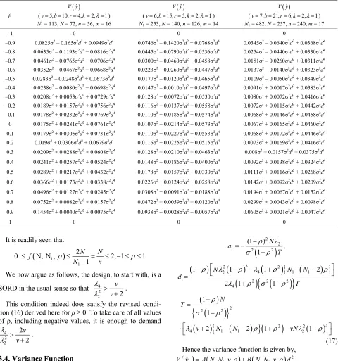
Table 2. Variance of the estim v ≤8 ,

2, 1

ated response for the factors3 ≤ when r = 3λ.

ρ

 ˆ

V y

(v4,b6,r3,k 

25, m =

)

N1 = 51, N = 27, n = 2

 ˆ

V y

(v7,b7,r3,k3,1)

N1 = 113, N = 57, n = 56, m = 1

–1  0  0 

–0.9  + 0.0350 σ2 _–

.8  + 0.0632 σ2 _–

  + 0.0815 σ2 _{– 0.050}

.6  + 0.0928 0365σ2 _–

.5  + 0.1004 289σ2 _–

.4  + 0.1065 241σ2 ₊

.3  + 0.1113 209σ2 ₊

.2  + 0.1145 190σ2 ₊

.1  + 0.1155 σ2 ₊

  + 0.1135 σ2 ₊

  2 2 2 2 4 2 2 2 .0 σ2_d4

 

0.2  1σ2_d4

 

0.3  0.0452σ2 _{+ 0.0492σ}2 _{+ 0.0893σ}2_d4

  0.0209σ2 _{+ 0.0285σ}2 _{+ 0.0468σ}2_d4

 

0.4  0.052 2 2 2 4

  0.0241 2 2 2 4

 

0.0622σ + 0.037 d + 0.0631σd4

  0.0289σ + 0.021 d + 0.0335σd4

 

0.0242σ2 _{– 0.0390σ}2_d2 _σ2_d4

  0.1400 0.1820σ2_d2 _{+ 0.0677σ}2_d4

 

–0 0.0413σ2 _{– 0.0630σ}2_d2 _σ2_d4

  0.0745 0.0890σ2_d2 _{+ 0.0445σ}2_d4

 

–0.7 0.0487σ – 0.0660σd

2 2 2

2 2 2 _σd

  0.0494

2 4

2 4 _{0σd + 0.0396σd}

 

2 2 2 4

2 2 2 4

–0 0.0493σ – 0.0540σd σd  0. 0.0260σd + 0.0405σd 

–0 0.0468σ2 _{– 0.0340σ}2_d2 _σ2_d4

  0.0 0.0100σ2_d2 _{+ 0.0437σ}2_d4

 

–0 0.0434σ2 _{– 0.0130σ}2_d2 _σ2_d4

  0.0 0.0031σ2_d2 _{+ 0.0478σ}2_d4

 

–0 0.0404σ2 _{+ 0.0069σ}2_d2 _σ2_d4

  0.0 0.0132σ2_d2 _{+ 0.0520σ}2_d4

 

–0 0.0382σ2 _{+ 0.0240σ}2_d2 _σ2_d4

  0.0 0.0209σ2_d2 _{+ 0.0553σ}2_d4

 

–0 0.0371σ2 _{+ 0.0373σ}2_d2 _σ2_d4

  0.0179 0.0266σ2_d2 _{+ 0.0573σ}2_d4

 

0 0.0370σ2 _{+ 0.0463σ}2_d2 _σ2_d4  _{0.0175 0.0300σ}2_d2 _{+ 0.0575σ}2_d4 

0.1 0.0382σ + 0.0510σd + 0.1083σd  0.0179σ + 0.0313σd + 0

0.0408σ2 _{+ 0.0518σ}2_d2 _{+ 0.1001σ}2_d4

  0.0190σ2 _{+ 0.0307σ}2_d2 _{+ 0.052}

557

d2 _d2

σ + 0.0442σd + 0.0767σ

2 2 2 2

2_{d σ + 0.0252σd + 0.0405}

2 2 2 2

σ2_d

0.5  6σ 1σ

0.6  0.0782σ2 _{+ 0.0300σ}2_d2 _{+ 0.0493σ}2_d4

  0.0366σ2 _{+ 0.0167σ}2_d2 _{+ 0.0262σ}2_d4

 

0.7  0.1045σ2 _{+ 0.0222σ}2_d2 _{+ 0.0358σ}2_d4

  0.0496σ2 _{+ 0.0123σ}2_d2 _{+ 0.0190σ}2_d4

 

0.8  0.1541σ2 _{+ 0.0145σ}2_d2 _{+ 0.0229σ}2_d4

  0.0752σ2 _{+ 0.0079σ}2_d2 _{+ 0.0122σ}2_d4

 

0.9  0.2759σ2 _{+ 0.0072σ}2_d2 _{+ 0.0109σ}2_d4

  0.1454σ2 _{+ 0.0038σ}2_d2 _{+ 0.0058σ}2_d4

 

1  0  0 

  ( ) 4 4

1

2 iu u

x r 4

N

2 3 ,

t k _ t v_{  N}







2 2

N

  ( ) 4

2t k 2t v _N ,

4 1

iu ju u

x x     







Using the above relations, for the newly constructed desi e get the follo

1

2 (

gn, w wing:

  ) 2

2

N

1 2

iu u

x r t k _2t v _{ N} , 





1 4

N

t k ₂t v( ) 4 _{3N ,}

4 2

x r 1 iu

u

 

 



1 2 2

N

iu ju





  ( ) 4 4 2t k 2t v

1

u

x x    N ( 

The results are given in Table 3

(These expression follow easi 



14)

.

ly from the definition of points sets generated from BIBD and the consequent multiplication with factorial combinations as explained in Raghavarao [7], pp. 298-300)

Using (5) and (12), (13), (14) the design p ameters of the newly constructed design are the following:

ir

ar

















2 2

2 4

(1 ) (1 )

,

N N

0 _{2 2 2 2}

1 1

2 2

2 1

a f

N N

e

4 (1 ) 1 (1 )

2 ₁ 2 ,_c 2 ₁ 2

   

   

   

   

 

 

 

(15)

Using (15) a





 

nd noting













1 1 2

N N

v00 ₂

1 2 1

 

  

,

the expression

 



2 2 _{v f} a0 

c  v00 simplifies to

























3

2 2

1

2

1 v

 2 2

2

2 1

2 1  N4 vN 

1 1

N N

 

 

 

  

 

 _   _

Hence the n above

de-signis

on-singularity condition of the

















3 1 4

2 2

2 1

1

2 2 1

N v

v N N

 

  

 _ 

 



 _    _

Let f (N, N1, ρ) =

















(16)

 3

2

1 1

1

2 1

N

N N



 

 

 

    _

[image:7.595.59.539.102.615.2]

Table 3. Variance of the timated response for the factors3 ≤v ≤8 , when r > 3λ.

 ˆ

V y

4, 2,

r k

es



ρ _{(v 5,b 10, 1}



ˆ

V y

5, 2,

r k

(v 6,b 15, 1



 

N1= 113, N

 

= 72, n = 56, m

 ) = 16



   

 ˆ

V y

1,r 6,k 2, 1

 ) (v 7,b 2

N1= 253, N = 140, n = 126, m = 14



   )

m = 17

 

N1= 482, N = 257, n = 240,

–1  0  0  0 

–0.9  0.0825σ2 _{– 0.165σ}2_d2 _{+ 0.0949σ}2_d4

  0.0746σ2 _{– 0.1420σ}2_d2 _{+ 0.0768σ}2_d4

  0.0345σ2 _{– 0.0640σ}2_d2 _{+ 0.0368σ}2_d4

 

.0790σ2_d2 _{+ 0.0536σ}2_d4

  0.0254σ2 _{– 0.0440σ}2_d2 _{+ 0.0330σ}2_d4

.0460σ2 2 2 4 2 2 2 2 4

.026

.0673σ2_d4`

  0.0177σ2 _{– 0.01 465σ}2_d4

  0.0109σ2 _{– 0.0050σ}2_d2 _{+ 0.0349σ}2_d4

 

.0010σ2_d2 _{+ 0.0497σ}2_d4

  0.0091σ2 _{+ 0.0017σ}2_d2 _{+ 0.0383σ}2_d4

 

0.0128σ2 _{+ 0.0072σ}2_d2 _{+ 0.0530σ}2_d4

  0.0080σ2 _{+ 0.0072σ}2_d2 _{+ 0.041}

–0.2  0.0189σ2 _{+ 0.0157σ}2_d2 _{+ 0.0756σ}2_d4

  0.0116σ2 _{+ 0.0137σ}2_d2 _{+ 0.0558σ}2_d4

  0.0072σ2 _{+ 0.0115σ}2_d2 _{+ 0.0442σ}2_d4

 

–0.1  0.0178σ2 _{+ 0.0232σ}2_d2 _{+ 0.0769σ}2_d4

  0.0110σ2 _{+ 0.0185σ}2_d2 _{+ 0.0574σ}2_d4

  0.0068σ2 _{+ 0.0146σ}2_d2 _{+ 0.0458σ}2_d4

 

0  0.0175σ2 _{+ 0.0281σ}2_d2 _{+ 0.0761σ}2_d4  _.0214σ2_d2 _0.0067σ2 _{+ 0.0165σ}2_d2 _{+ 0.0460σ} 4 

0.1  0.0179σ2 _{+ 0.0305σ}2_d2 _{+ 0.0731σ}2_d4

  0.0110σ2 _{+ 0.0227σ}2_d2 _{+ 0.0553σ}2_d4

  0.0068σ2 _{+ 0.0172σ}2_d2 _{+ 0.0446σ}2_d4

 

0.2  0.019σ2 _{+ 0.0306σ}2_d2 _{+ 0.0679σ}2_d4

  0.0116σ2 _{+ 0.0225σ}2_d2 _{+ 0.0515σ}2_d4

  0.0073σ2 _{+ 0.0169σ}2_d2 _{+ 0.0416σ}2_d4

 

0.3  0.0209σ2 _{+ 7σ}2_d2 _{+ 0.0375σ}2_d4

 

0.4  0.0241σ2 _{+ 0.0257σ}2_d2 _{+ 0.0524σ}2_d4

  0.0148σ2 _{+ 0.0186σ}2_d2 _{+ 0.0400σ}2_d4

  0.0092σ2 _{+ 0.0138σ}2_d2 _{+ 0.0324σ}2_d4

 

0.0289σ2 _{+ 0.0217σ}2_{d + 0.0432} 2 4

  0.0178σ2 _{+ 0.0157σ}2_{d + 0.0330σ}2 4

  0.0111σ2 _{+ 0.0116σ}2_{d + 0.0268σ}2 4

 

0.6  0 4

 

0.0496σ2 _{+ 0.012 d}2 _{+ 0.0245σ}2_d4

  0.0308σ2 _{+ 0.009} 2_d2 _{+ 0.0188σ}2_d4

  0.0194σ2 _{+ 0.006} 2_d2 _{+ 0.0152σ}2_d4

 

–0.8  0.0635σ2 _{– 0.1193σ}2_d2 _{+ 0.0816σ}2_d4

  0.0445σ2 _{– 0}

–0.7  0.0461σ2 _{– 0.0765σ}2_d2 _{+ 0.0706σ}2_d4

  0.0300σ2 _{– 0}

–0.6  0.0352σ2 _{– 0.0467σ}2_d2 _{+ 0.0668σ}2_d4

  0.0223σ2 _{– 0}

–0.5  0.0283σ2 _{– 0.0248σ}2_d2 _{+ 0}

 

d + 0.0458σd  0.0181σ – 0.0260σd + 0.0311σd 

0σ2_d2 _{+ 0.0447σ}2_d4

  0.0137σ2 _{– 0.0140σ}2_d2 _{+ 0.0323σ}2_d4

 

20σ2_d2 _{+ 0.0}

–0.4  0.0238σ2 _{– 0.0080σ}2_d2 _{+ 0.0698σ}2_d4

  0.0147σ2 _{– 0}

–0.3  0.0208σ2 _{+ 0.0053σ}2_d2 _{+ 0.0729σ}2_d4

  6σ2_d4

 

0.0107σ2 _{+ 0 + 0.0573σ}2_d4  2_d

0.0288σ2_d2 _{+ 0.0608σ}2_d4

  0.0128σ2 _{+ 0.0210σ}2_d2 _{+ 0.0463σ}2_d4

  0.008σ2 _{+ 0.015}

0.5  2 σd 2 _d 2 _d

.0366σ2 _{+ 0.0173σ}2_d2 _{+ 0.0338σ}2_{d 0.0226σ}2 _{+ 0.0124σ}2_d2 _{+ 0.0258σ}2_d4

  0.0142σ2 _{+ 0.0092σ}2_d2 _{+ 0.0209σ}2_d4

 

0.7  7σ2 _{1σ 7σ}

0.8  0.0752σ2 _{+ 0.0082σ}2_d2 _{+ 0.0157σ}2_d4  _0.0472σ2 _{+ 0.0059σ}2_d2 _{+ 0.0120σ}2_d4  _0.0299σ2 _{+ 0.0043σ}2_d2 _{+ 0.0098σ}2_d4 

0.9  0.1454σ2 _{+ 0.0040σ}2_d2 _{+ 0.0075σ}2_d4

  0.0938σ2 _{+ 0.0028σ}2_d2 _{+ 0.0057σ}2_d4

  0.0605σ2 _{+ 0.0021σ}2_d2 _{+ 0.0047σ}2_d4

 

1 0  0  0 

readi

It is ly seen that



N, N , 2,1 



   

1 1

N  n

0  f 1

ow start w

SORD in th

2N N _1

We n argue as follows, the design, to ith, is a e usual sense so that 4 _ v

2

2 2

.

cond revise

tio 6) de re of a

of nclud gh to

v

 

This ition indeed does satisfy the d condi- n (1 rived here for ρ≥ 0. To take ca ll values

ρ, i ing negative values, it is enou demand 4 _

2 _v

2 2

2 v 

 

3.4 arian

The varianc nder t

correlated structure constructed by the above method is btained by using (7), and (16) and noting the following:















.

. V ce Function

e function of SORDWCE u he auto- o



N1

v00 ₂1 ₂

2 1

1

N  

 

 











 





2 2 1

v N ₄

00

2 ₁ 2 v

T





2 (1 ) N ₂

2 ₁ 2 _T, 1

a  

 

  























 







3

1 N 2

2 2

2 4 1 2 1

4 1 1

1 _{2 2 2}

1 T

1 N N

d   



  

  

 _ 

 _     _



 





















4 v 2 N1







2

1

N 2





1 



vN₂



1 



2 ₁ 2

 

3

2 2

1 N

T 

 _{ } 

_     _

7) ance fu

(1 Hence the vari nction is given by,

 









2

1

, , ,

B N N v  d 

,

1

1

, , , ,

v N v

 

where,

4

)d

, ˆ_x

V y A N N

( ,

C N  say,

















 

 

 









 

2 2 2

0

2 1 _ˆ

1

v

V T

4 1

1 , , ,

A N N v    

1

 

  

 

























2 2

2

1 ₂ 4

2 1

1

, , , 2 1

1

B N N v v

N T

 

  

 



 

 _   _











 











 

i 2Cov



ˆ ˆ0, ii



2

2 2

1 1 2 2 1 1 2 1 ˆ

N  N   N  v    V    



















_



_









 

3 2

2

4 1

1 1 2 ( 1) 1

1 _ˆ

λ 1 ii

v N N N v

V

2 2  2   

4 1 1 2

1 , , ,

C N N v 

2N T

  



 _{      } 

 _{ }







1

3

2 2

2 1 .

T

vN 

 _ 

 

thod with the h the help of BIBD. Consider the BIBD (v = 7, b = 7, r = 3, k = 3, λ = 1).Here we have, N = 57, N1 = 113, n = m = 1.

1 1 1

2 4 2 2

4 1

8

N N N

ju u

where

















4 v 2 1 N1 N1 2

  

     

Example: We illustrate the above me construction of RSORD for 7-factors w



it 56,

2 4

1 1

24 , 24 3 ,

iu iu iu

u u

x N x N x x N



 



Plan of B

B1  1  2  4 

 

   





BI D:

B2  2  3  5 

  3  4  6 

B4  4  5  7 

B5  5  6  1 

B6  6  7  2 

B7  7  1  3 

B3

The design (denoted by d0) is displayed here for rea y ference (column being runs).

d0 1 2 3 4 5 6 7 8 9 10 11 12 13 14 15 16 17 18 19 20

d re

x1 0 1 0 1 0 1 0 1 0 –1 0 –1 0 –1 0 –1 0 0 0 0

x2 0 1 0 1 0 –1 0 –1 0 1 0 1 0 –1 0 –1 0 1 0 1

x3 0 0 0 0 0 0 0 0 0 0 0 0 0 0 0 0 0 1 0 1

x4 0 1 0 –1 0 1 0 –1 0 1 0 –1 0 1 0 –1 0 0 0 0

x5 0 0 0 0 0 0 0 0 0 0 0 0 0 0 0 0 0 1 0 –1

x6 0 0 0 0 0 0 0 0 0 0 0 0 0 0 0 0 0 0 0 0

x7 0 0 0 0 0 0 0 0 0 0 0 0 0 0 0 0 0 0 0 0

d0 21 22 23 24 25 26 27 28 29 30 31 32 33 34 35 36 37 38 39 40

x1 0 0 0 0 0 0 0 0 0 0 0 0 0 0 0 0 0 0 0 0

x2 0 1 0 1 0 –1 0 –1 0 –1 0 0 0 0 0 0 0 0

x 0 0 0 1 0 1 0 1

0 0 0 1 0 –1 0 –1

0 0 0 0 0 0 0 0

0 0 0 0 –1 0 1 0 –1

0 0 0 0 0 0 0 0 0 0

–1 0

3 0 –1 0 –1 0 1 0 1 0 –1

x4 0 0 0 0 0 0 0 0 0 0

x5 0 1 0 –1 0 1 0 –1 0 1

x6 0 0 0 0 0 0 0 0 0

x7 0 0 0 0 0 0 0 0

–1 1

0 1

–1 0

0 1

0 0

d0 41 42 43 44 45 46 47 48 49 0 51 525 53 54 55 56 57 58 59

x1 0 0 0 0 0 0 0 0 0 0 0 0 0 0 0 0 0 0 0

x2 0 0 0 0 0 0 0 0 0 0 0 0 0 0 0 0 0 0 0

x3 0 –1 0 –1 0 –1 0 –1 0 0 0 0 0 0 0 0 0 0 0

1 0 –1 0 –1 0 1 0 1 0 1 0 1 0 –

0 0 0 0 0 0 1 0 1 0 –1 –1 0 1

0 1 0 –1 0 0 0 0 0 0 0 0 0 0

0 0 0 0 0 0 1 0 –1 0 1 0 –1 0 1

x4 0 1 0 1 0

x5 0 0 0 0 0

x6 0 1 0 –1 0

x7 0 0 0 0

2 3 64 65 66 67 68 69 70 71 72 7 7 7 7 7

d0 60 61 6 6 3 4 5 6 7 78

x1 0 0 0 0 0 1 0 1 0 1 0 1 0 –1 0 –1 0 –1 0

x2 0 0 0 0 0 0 0 0 0 0 0 0 0 0 0 0 0

x3 0 0 0 0 0 0 0 0 0 0 0 0 0 0 0 0 0 0 0

0 0 0 0 0 0 0

1 0 1 0 1 0 –1 0 –1 0 1 0 1 0 –1

1 0 –1 0 1 0 –1 0 1 0 –1 0 1

x7 –1 0 1 0 –1 0 0 0 0 0 0 0 0 0 0 0 0 0 0

0 0

x4 –1 0 –1 0 –1 0 0 0 0 0 0 0

x5 1 0 – 0 –1