Sinusoidal Time Dependent Power Series Solution to Modified Duffing Equation

ISSN Online: 2161-1211 ISSN Print: 2161-1203

DOI: 10.4236/ajcm.2018.83021 Sep. 29, 2018 259 American Journal of Computational Mathematics

Sinusoidal Time-Dependent Power Series

Solution to Modified Duffing Equation

Haiduke Sarafian

The Pennsylvania State University, University College, York, PA, USA

Abstract

Duffing equation, _{x t}

( ) ( )

_{+x t +}

_ε

_{x t}3

( )

_{=0, has a standard well-known exact} solution [1]. Approximate solutions to this equation also are available [2]. Reference [3] [4] introduces a sinusoidal time-dependent Power Series tion. Applying this method successfully we investigate the approximate solu-tion of the modified Duffing equasolu-tions, _{x t}

( ) ( )

_{+x t +}

_ε

_{x t}n

( )

₌0_{, for n = 4}

and 5. Symbolic manipulative utilities of a Computer Algebra System (CAS) specifically Mathematica [5] extensively is used investigating the results.

Keywords

Duffing Equation, Modified Duffing Equation, Nonlinear Quartic and Quintic Terms, Mathematica

1. Introduction

There are numerous scientific and engineering phenomena encountering oscil-lations. The simplest oscillations are described by a generic linear differential equation,

ξ



( ) ( )

t +

ξ

t =0, where ξ(t) is the time-dependent quantity of interest. For instance, ξ(t) could describe the oscillation of the electric charge, q(t), in an LC series electric circuit, or it may describe oscillating coordinate, x(t), of a particle under the influence of a linear force. This equation modifies if one includes retard-ing,

ξ



( )

t , term and external forces, f(t), resulting,

ξ



( ) ( ) ( )

t +

ξ

 t +

ξ

t = f

( )

t , preserving its linearity. Motivation of considering Duffing type equation stems from the fact that the nonlinearity implicitly is embedded in the former equation. For instance, for a mechanical system one might encounter an equation such as, θ

( )

t +sin_θ

( )

t _=0. Replacing the second term with its approximate form yields,

( ) ( )

1 3

( )

₀

6

t t t

θ

 +

θ

−

θ

 . Meaning Duffing equation is implicit to How to cite this paper: Sarafian, H. (2018)

Sinusoidal Time-Dependent Power Series Solution to Modified Duffing Equation. American Journal of Computational Ma-thematics, 8, 259-268.

https://doi.org/10.4236/ajcm.2018.83021

Received: September 1, 2018 Accepted: September 26, 2018 Published: September 29, 2018

Copyright © 2018 by author and Scientific Research Publishing Inc. This work is licensed under the Creative Commons Attribution International License (CC BY 4.0).

DOI: 10.4236/ajcm.2018.83021 260 American Journal of Computational Mathematics oscillating motion. As in another instance a nonlinear force may result an equa-tion of moequa-tion, _{x t}

( ) ( )

_{+x t +}

_

_x3

( )

_{t =0. Solving these ODEs is a prime interest.} Aside searching for their exact solutions [1] various approximation methods have been sought for [2]. Method introduced in [3] [4] is the most updated ap-proximation solution of the Duffing equation.

It is one of the objectives of our investigation to examine the validity of the method [3] [4] solving modified Duffing equation. Modified Duffing equations are the ones that replace the cubic term with either quartic or quintic term.

With these motivations we craft this note; it is composed of four sections. Aside the Introduction, in Section 2 first we brief on the exact and Power Series solution of Duffing equation. Section 3 is the results. Section 4 is the conclusions embodying suggestions for extensions and modifications.

2. A Brief Review of Exact and Power Series Solution of

Duffing Equation

To establish the basis, we begin with the standard Duffing equation,

( ) ( )

3

( )

₀

x t +x t + x t =





, (1)

Its exact solution with two initial conditions, x

( )

0 =a1 and x

( )

0 =0, is [1],

( )

1

[ ]

,

x t =a cn u k _,

₍₂₎

where, u a t= 2 , with a2 and k subject to,

2

2 1 1

a = +a  and

₍

12

₎

2 1

2 1

a k

a =

+





,

(3)

In Equation (2), cn

[

ζ,m

]

, is the Jacobi elliptic function, cn

[

ζ,m

]

=cosϕ_, with _ϕ=F−1_F

[

_{ϕ,m m}

]

_{, }

 , where, F

[

ϕ,m

]

is subject to [6] [7],

[

]

2 2 0

d ,

1 sin

F m

m

ϕ

_ϑ

ϕ

ϑ

= −

∫

,

(4)

As one expects Duffing equation describes oscillations. The severity of devia-tion of the oscilladevia-tions given by Duffing equadevia-tion from the corresponding linear case (ϵ = 0) depends on the value of ϵ. The value of ϵ implicitly impacts the period of the oscillations given by,

2

4 π_,

2

T F k

a

 

= _{ }

 .

Having established the fundamentals now we cross-examine the accuracy of the Power Series approximation Method outlined in [3] [4].

sinu-DOI: 10.4236/ajcm.2018.83021 261 American Journal of Computational Mathematics soidal functions of the polynomial are the same. The absence of dissipative term,

( )

x t , in Duffing equation warrants the conservativeness of energy of the sys-tem leading to a unique value for the frequency of the polynomial. As is true in general, the accuracy of the series method is being controlled by the order of the polynomial—for the case on hand the order depends implicitly to the coefficient of the nonlinear term, ϵ.

As is outlined in [3] [4] a Power Series solves the Equation (1),

( )

[ ]

( )

1

1

sin

N _n

n

x t a n ωt − =

=

∑

_ _ ,

(5)

A change of variable, τ=sin

( )

ωt _{, replaces t,} t≥0 , with − ≤ ≤ +1 τ 1 yielding Equation (1),

(

)

2

( )

( ) ( )

( )

2 2 2 3

2

d d

1 0

d

d x x x x

ω τ τ ω τ τ τ τ

τ τ

− − + + = ,

(6)

Noticing significant changes; e.g. Equation (6) gained a dissipative term with a τ-dependent coefficient.

Realizing,

( )

[ ]

1 1

N n n

x τ a nτ − =

=

∑

and 3

( )

[ ]

1

1

N n n

x τ b n τ − =

=

∑

, Equation (6) yields

the recurrence relationship between the coefficients,

[

]

[ ]

(

₍

)

₎

[ ]

2 2 2 1 1 2 1

a n n b n

a n n n ω ω  _{− − −}   + = + 

, for n=1,2,3, (7)

For the chosen initial conditions, x t

[

=0

]

= =A a

[ ]

1 _and x t

[

=0

]

= =0 a

[ ]

2 , Equation (7) gives the remaining coefficients yielding the solution of Equation (5). Because of the second initial condition all the even expansion coefficients are zero limiting the polynomial to even powers of the base only. More on this in Conclusion section.

The lack of dissipative term in Duffing equation signifies the conservation of energy. The energy of the system, E T V= + , stays constant. The T and V for a point-like particle of mass m under the action of a nonlinear force, _{F k x= } 3_, respectively are,

( )

2

1 2

T = mx t and 1 2

( )

1 4

( )

2 4

V = kx t + k x t , (8) Equation (8) for the generic case, m k= =1 _{is associated with the Lagrangian,}

( )

,

L x x = −T V. Applying Euler-Lagrange equation, d 0 d

L L

t x x

∂ ₋∂ ₌

∂ ∂ , yields the equation of motion, Equation (1).

Utilizing the time independence of energy and implied initial conditions yields an equation conducive the needed, ω, in Equation (5).

The maximum potential energy occurs at t=0 when the particle is at maxi-mum distance from the equilibrium, i.e.

(

)

2 4

max 0 1₂ 1₄

V t= = A + A . The maxi-mum kinetic energy occurs when the particle passes the equilibrium,

(

)

( )

2

2 2

max 1₂ 1 _dd

T ω τ x τ

τ

 

= − _{ }

  , at

1 2

DOI: 10.4236/ajcm.2018.83021 262 American Journal of Computational Mathematics max max

T =V , (9) With these outlines we craft a Mathematica program leading the quantity of interest. For objectively chosen numeric values for initial displacement, A, stiff-ness, ϵ, we investigate the accuracy of the Power Series Method vs. the exact so-lution; these are given in Sect. 3.

3. Results

3.1. Solutions of Duffing Equation: Power Series, Exact, and Numeric

For the chosen value of A and ϵ the number of terms, N, in Equation (5) ought to be determined warrants the convergence of series. To compare our CAS ap-proach to [4] we set the values of

{ } {

A, = 1.0,2.0

}

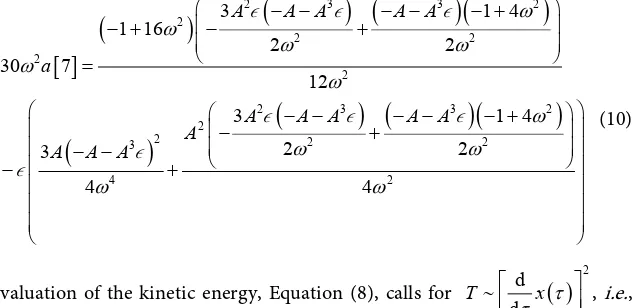
. By trial and error and the CPU run-time limitations, we set N = 28. As we pointed out because other than the first term only the even powers of sin(ωt) are contributing, evaluation of x(t), Equation (5), requires determination of fourteen expansion coefficients. Recur-sive relationship between the coefficients, Equation (7), makes the symbolic ex-pressions massive. For instance, a [7], is,

[ ]

(

)

(

) (

)(

)

(

)

(

) (

)(

)

2 3 3 2

2

2 2

2

2

2 3 3 2

2

2 2 2

3

4 2

3 1 4

1 16

2 2

30 7

12

3 1 4

2 2

3

4 4

A A A A A

a

A A A A A

A A A A

ω ω ω ω ω ω ω ω ω ω ω  _{− − − − − +}    − + − +     =   − − − − − +   − +   _{− −}       − +                 (10)

Evaluation of the kinetic energy, Equation (8), calls for d

( )

2 d

T x τ τ

 

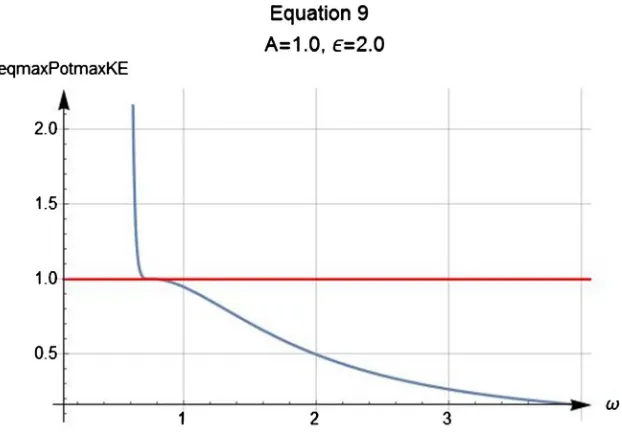
∼ _ _ , i.e., 169 symbolic expressions are to be called upon. Each term is a complicated ω-dependent, one of these terms is the squared of Equation (10)! Justifiably we suppressed writing it down. Display of the kinetic and potential energies vs. ω and their intersection is shown in Figure 1. Figure 1 helps guesstimating the abscissa of the intersection.

Applying the FindRoot utility of Mathematica at about the guesstimated ab-scissa gives the exact root value of Equation (9), ω = 0.7992207. Reference [4] uses eighty terms, e.g. N = 80 evaluating ω. In our case, N = 28, yields an ac-ceptable value.

[image:4.595.222.540.331.485.2]

DOI: 10.4236/ajcm.2018.83021 263 American Journal of Computational Mathematics Having the values of expansion coefficients and ω we plot the t-dependent po-sition x(t) given by Equation (5). This is shown in Figure 2 in Black.

[image:5.595.219.530.125.343.2]

Duffing equation, Equation (1) as discussed has an exact solution [1]. The

[image:5.595.68.538.403.696.2]

Figure 1. Display of the maximum potential (Red) and kinetic (Blue) energies vs. ω for

{ } {

A,_ = 1.0,2.0

}

_{with N = 28.}

Table 1. The first fourteen expansion coefficients of Equation (5) for

{ } {

A,_ = 1.0,2.0

}

_{with N = 28.}

n 1 3 5 7 9 11 13 15 17 19 21 23 25 27

a[n] 1. −2.3482 1.3617 −1.4977 1.1270 −1.0472 0.8581 −0.7593 0.6390 −0.5568 0.4727 −0.4099 0.3489 −0.3021

DOI: 10.4236/ajcm.2018.83021 264 American Journal of Computational Mathematics solution may be expressed in terms of the built in Mathematica library JacobiCN function,

( )

(

)

2 2 2 2 1 , 2 1 A x t AJacobiCN A t

A     =          +  ₊   _{ }  

 . Figure 2 displays this function

in Green. Although our numeric computation applying Power Series includes “only” 14-terms its accuracy is as close as the exact solution. We further our in-vestigation applying Mathematica NDSolve solving Equation (1) numerically. NDSolve uses one of the common numeric methods of Implicit Runge Kutta or StiffnessSwitching which is a combination of the explicit and implicit methods solving the equation. The numeric solution perfectly matches the exact solution. The Green curve is the exact solution, it indistinguishably overlaps with the nu-meric solution. The black curve is the Power Series solution.

Despite the fact that the number of terms in Equation (5) is limited to fourteen the agreement between the exact/numeric and approximate results are quite ac-ceptable. As shown in Figure 2, within the long range of the t-axis the positive amplitude of the approximated method overlaps the exact amplitude and over-estimates the negative ones. This can be rectified if a greater number of terms could be included in Equation (5). On the other hand, the period of all three methods is in very good agreements.

As shown in Figure 2, the oscillation has a period of about four. Applying the value of ω the period is

( ) (

2π 2 0.799227×

)

=3.92_{. For the exact solution as}

pointed out in Sect. 2 the period is, 4 1 4

3 3

T = K_ _=

  , where

[ ]

π 2 2 2 0 1 _d 1 sin K m

m ϑ ϑ

= −

∫

; these two are in good agreement.

3.2. Nonlinear Quartic Term

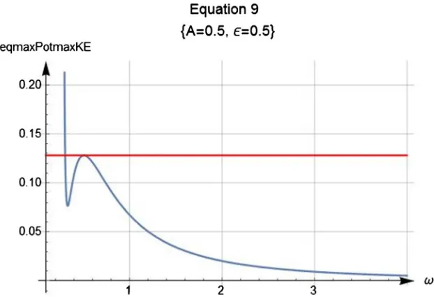
In this subsection we investigate the validity of the Power Series Method for a modified Duffing equation by replacing the ϵx3_{(t) with ϵx}4_{(t). Being practical for} the case on hand we consider

{

x

[ ]

0 ,

}

=

{

0.5,0.5

}

. By trial and error, we set the number of the terms, N, in Equation (5) to 20. Based on what we have discussed the non-zero terms limits the contributing terms to eleven. For the quartic term the maximum potential energy is,

(

)

2 5

max 0 1₂ 1₅

V t= = A +



A . Plotting the kinetic

and potential energies vs. ω their intersection abscissa according to Equation (9) yields ω. This is shown in Figure 3.

Figure 3 assists evaluating the exact abscissa of the intersection; ω = 0.510225. Utilizing ω, we tabulate the expansion coefficients; these are given in Table 2.

Numeric values of Table 2 are based on utilizing the recurrence relationship between the coefficients given by Equation (7).

[image:7.595.218.529.110.323.2]

DOI: 10.4236/ajcm.2018.83021 265 American Journal of Computational Mathematics For chosen parameters the results are in good agreement; noting analytic solu-tion for the case on hand is not available.

[image:7.595.210.535.393.690.2]

Figure 3. Display of the maximum potential (Red) and kinetic (Blue) energies vs. ω for

{ } {

A, = 0.5,0.5

}

for N = 20.

Table 2. The first ten expansion coefficients of Equation (5) for

{ } {

A, = 0.5,0.5

}

with N = 20.

n 1 3 5 7 9 11 13 15 17 19

a[n] 0.5 −1.0203 0.0681 −0.0745 0.0384 −0.0119 0.0047 −0.0037 0.0001 −0.0012

DOI: 10.4236/ajcm.2018.83021 266 American Journal of Computational Mathematics

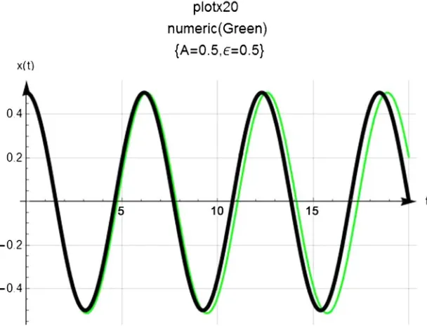
Figure 4 compares the numeric solution vs. the Power Series Method. Figure caption indicates the parameters. As shown plots are acceptably comparable. The accuracy of the Power Series Method could have been increased had we could include a greater number of terms. More on this in Conclusion section.

3.3. Nonlinear Quintic Term

In this subsection similar to Sect. 3.2 we investigate the validity of the Power Se-ries Method for solving a modified Duffing equation with ϵx5_{(t). We consider,}

{ } {

A, = 0.5,0.5

}

. With trial and error, we set the number of the terms, N, in Equation (5) to 20. The maximum potential energy for the case on hand is

(

)

2 6

max 0 1₂ 1₆

V t= = A +



A . We skip displaying the kinetic and potential energies

vs. ω as is similar to Figure 1 and Figure 3. Suffices noting the intersection of these two curves yields, ω = 0.506614.

[image:8.595.221.525.458.690.2]

The numeric solution is the output of NDSolve. The equation on hand likewise to the previous case, Sect. 3.2, has no exact solution.

Figure 5 compares the numeric solution vs. the Power Series Method. Figure caption indicates the parameters. As shown oscillations are acceptably compara-ble. The accuracy of the Power Series Method would increase if a greater number of terms could be included. More on this in Conclusion section.

4. Conclusions and Suggestions

We applied a Computer Algebra System (CAS), Mathematica examining its ap-plicability to solving Duffing equation utilizing the Power Series Method. We have shown with Mathematica we are able producing the numeric results of [4].

DOI: 10.4236/ajcm.2018.83021 267 American Journal of Computational Mathematics Moreover, we extend the calculation to symbolic domain; this is not included in [4]. Applying Mathematica we then successfully explore its applicability to solv-ing modified Duffsolv-ing equations embodysolv-ing nonlinear quartic and quintic terms.

For Duffing equation computation power of a laptop with a double processor prevents increasing the number of the terms evaluating Equation (5) to achieve accuracies beyond what is reported. Equation (7) is a recursive relationship be-tween the expansion coefficients embodying b[n]. In general we write

[ ]

1

[ ]

1

1 1

m

N N

n n

n n

a n

τ

− b n

τ

−

= =

  ₌

 



∑



∑

, for m=2,3,4,; for Duffing case, m = 3. We notice replacing N = 28 with 30 drastically increases the number of b[n] greatly elongating the computation run-time crashing the computer. Number of terms in [4] is eighty, this is not achievable for our symbolic calculation approach.

Extension of the current investigation. A curious reader may inquire: “What are the implications to numeric and symbolic solutions of the Duffing, modified Duffing equations embodying quartic and quintic terms if the second initial condition is replaced with, x t

[

=0

]

≠0?” Quantification of the answer would require accessibility to a much more powerful computer as it would encounter lengthy symbolic calculation.

A note to the readers: Figures and calculations in this article are carried out utilizing Mathematica resources [5] [8]. Readers may also find [9] resourceful addressing related issues.

Acknowledgements

Motivation of this investigation stems from the questions that the author put to the presenter of “Power Series solution for strongly non-linear conservative os-cillators” at “6th _{International Physics Conference”, Athens/Greece, July 2018.} One of the questions was “...has the Power Series Method been tested for nonli-near terms higher than three?” the answer was negative. The author initiated the investigation crafting this note. The author thanks Professor Mazen I. Qaisi for private communications and appreciates the support staff of Wolfram Research Inc. for consulting the issues concerning the numeric algorithm used in NDSolve.

Conflicts of Interest

The authors declare no conflicts of interest regarding the publication of this pa-per.

References

[1] Salas, A. and Castillo, J. (2014) Exact Solution to Duffing Equation and the Pendu-lum Equation. Exact Mathematical Sciences, 8, 8781-8789.

[2] Rand, R. (2005) Lecture Notes on Nonlinear Vibrations.

http://www.tam.cornell.edu/randdocs/

DOI: 10.4236/ajcm.2018.83021 268 American Journal of Computational Mathematics

[4] Qaisi, I. (2018) Presented Note at “6th International Physics Conference”. 6th In-ternational Physics Conference, Athens, July 2018.

[5] Wolfram, S. (1996) Mathematica Book. 3rd Edition, Cambridge University Press, Cambridge.

[6] Mathworld. http://mathworld.wolfram.com/JacobiEllipticFunctions.html

[7] Abramowitz, M. and Stegun, I. (1970) Handbook of Mathematical Functions with Formulas, Graphs, and Mathematical Tables. Dover Publications, Inc., New York. [8] Sarafian, H. (2015) Mathematica Graphics Example Book for Beginners. Scientific

Research Publishing, Wuhan.