Numerical Approach of Network Problems in Optimal
Mass Transportation
Lamine Ndiaye1, Babacar Mbaye Ndiaye1, Pierre Mendy1, Diaraf Seck1,2
1Laboratory of Mathematics of Decision and Numerical Analysis (LMDAN), FASEG, University of Cheikh Anta Diop, Dakar, Senegal
2Unité Mixte Internationale, UMMISCO, Institut de Recherche pour le Développement, Bondy, France Email: [email protected]
Received February 13,2012; revised March 23, 2012; accepted March 31, 2012
ABSTRACT
In this paper, we focus on the theoretical and numerical aspects of network problems. For an illustration, we consider the urban traffic problems. And our effort is concentrated on the numerical questions to locate the optimal network in a given domain (for example a town). Mainly, our aim is to find the network so as the distance between the population position and the network is minimized. Another problem that we are interested is to give an numerical approach of the Monge and Kantorovitch problems. In the literature, many formulations (see for example [1-4]) have not yet practical applications which deal with the permutation of points. Let us mention interesting numerical works due to E. Oudet begun since at least in 2002. He used genetic algorithms to identify optimal network (see [5]). In this paper we intro-duce a new reformulation of the problem by introducing permutations . And some examples, based on realistic sce-narios, are solved.
Keywords: Optimal Mass Transportation; Network; Urban Traffic; Monge-Kantorovich Problem; Global Optimization
1. Introduction
In this paper we present some models of urban planning. These models are examples of applications in mass trans- portation theory. They describe how to optimize the de- sign of urban structures and their management under rea- listic assumptions. The paper is organized as follows: in Section 2 we present at first some urban planning models and preliminaries. The Section 3 is devoted to the appro- ximation of the models; and numerical simulations that are our main results. Finally, summary and conclusions are presented in Section 4.
2. Preliminaries and Mathematical Modeling
Given two distributions and on with equal total mass, the classical generic Monge transportation pro- blem consists in finding among all the maps d
verifying for any measurable set in , those which solve the minimization problem:
d
T:d
1
=T B B
d
minTI T , I T =
dc x T x, d x .These maps are said to be transportation maps; they transport a measure (quantity) to a measure .
For the existence of solutions, we recommend to see [6-10]. We invite the reader to see the books written in this topic by Villani [11,12] for additional information.
In particularly Sudakov have studied in [13] the exis- tence of optimal map transportation when
, =c x y xy and is absolutely continuous with respect to the Lebesgue measure d.
For studying the many cases where the Monge trans- portation problem doesn’t give a solution, Kantorovich considered the relaxed version of the Monge problem. In this framework, the transportation problem consists in finding among all admissible measures :dd
having and as marginals, those which solve the minimization problem
# #
1 2
, ,
= min d d , d , :π = ,π = .
MK c
c x y x y
The meaning of the following expressions # 1 π =
and # 2
π = is explained respectively as follows:
=
d
A A
and d =
A A
for any measurable subset A of d.
The Monge-Kantorovich problem obtained, depends only on the two distributions and , and the cost which may be a function of the path connecting
c x to
. y
design problem. When the unknown is the transportation network, we have an irrigation problem, that is an opti- mal design of public transportation networks.
We also mention the dynamic formulation of mass transportation given in [4,14,15] and generalized in [16]. In this framework, we consider that:
the space of measures acting is a time-space domain
= 0,1
Q where the urban area is a bounded Lipschitz open subset with outward normal vector n;
the mass density
t x, at the position x and timet is a Borel measure supported on Q , i.e.
,
b Q ; the velocity field v t x
, of a particle at
t x, is aBorel vectorial measures supported on Q;
the velocity field
t x, of the flow at
t x, is aBorel vectorial measures supported on Q
i e. .
, d
Q and defined by
b
t x, =
t x v,
t x, .The Monge-Kantorovich mass transportation problem consists in solving the following optimization problem:
min , : , , , d
b Q b Q
(1)with the constraints:
0= 0 on 0,1 ,
0, = 1, = ,
= 0 on 0,1 .
t divx
1
x x x x
n
(2)
where is an integral functional on the 1d-valued
measures defined on Q. Note that (2) is the continuity
equation of our mass transportation model.
2.1. Optimal Urban Design
In the models of optimal design of an urban area we con- sidered that
the urban area is a well known regular compact subset of d;
the total population and the total production are fixed data of the problem;
only the density of residents and the density of services are unknowns data of the problem. The aim is to find the density of residents and the density of services minimizing the transportation cost.
Principally there are two models for studying the op- timal urban design. The first one takes into account the following facts:
there is a transportation cost for moving from the re- sidential areas to the services poles;
people do not desire to live in areas where the density of population is too high;
services need to be concentrated as much as possible, in order to increase efficiency and decrease manage- ment costs.
The transportation cost will be described through a Monge-Kantorovich mass transportation model.
In particularly, we will take it as the -Wasserstein distance defined by:
p
1# #
1 2
, = min d ,
π = ,π = .
p d d p
p
W x y
x y :Taking into account the total unhappiness of residents due to high density of population, we define a penaliza- tion functional of the form
=
d if = d otherwise,h u x x u x
H
where u is the density of the population,
: 0, 0,
h is supposed to be convex, null at the origin and super linear (that is h t( )
t as t ). The increasing and diverging function
( )
h t t
t
repre-
sents the unhappiness to live in an area with population density . t
Thus we define a functional G
which penalizes sparse services. This functional is of the form:
=
if =otherwise,
i i i
i i
g a a
G x
where g: 0,
0,
is supposed to be concave,null with infinite slope at the origin (i.e. g t( )
t as
0
t ). Every single term g a
i in the sum above represents the cost for building and managing a service pole of size ai located at the point xi of . The Re-port
= i i
i
a P a
gP a is the productivity of pole of size
.
i
a
So in the first model, the optimal urban design pro- blem becomes the following optimization problem:
min , :
, probabilities on
p
W H G
(3)
In the second model the population transportation is considered as a flow, that is a vector field . The equilibrium condition is achieved when the emerg- ing flow is the excess of the demand in
2
:
K, i.e.
1
d n =
K
K n K
.the point x depends on the traffic intensity at x, i.e.
.k x g x
where g: 0,
0,
is an increasing function.Then, the transportation cost moving to is:
, = inf d : = and
= 0 on .
g
C g x x x
n
The problem (1) with the constraints (2) allows both to take into account the congestion effects by an appro- priated choice of the functionals and to widen the choice of unhappiness function and management cost function
h
g of the first model to the local lower semi- continuous functionals on
, d 1
b Q
.
For more details, we refer the interested reader to the several recent papers on the subject (see for instance [4, 14-17]).
2.2. Network Problems Applied to the Urban Transportation
In the models of optimal design of an urban area we con- sidered that
the urban area is a well known regular compact subset of d;
the density of residents and the density of ser- vices are two well known positives measures with equal mass.
The irrigation problem consists to find among all fea- sible structures (or feasible network) those that mini- mize the transportation cost
=
d
,
d
, ;I
c x y x yThe particular irrigation problem of the average dis- tance consists to find an optimal network opt for which the average distance for a citizen to reach the mos t nearby point of the network is minimal.
d
two
min
dist x, x d :x
is a feasible ne rk .
Theorem 1 For every there exists an optimal network
> 0
L
L
for the Optimization problem
1
min dist x, f x d :x connected and ( L
)d
main says for example a town.
pr
ical
Simulations
the blem
rst ap- proa rom this, we deduce a genera-
where 1 is the Hausdorff measure defined on . Notice that there are other proposition of functionals to be minimized.
For more details, we refer the interested reader to the several recent papers on the subject (see for instance [1-3, 18,19]).
Our aim is to concentrate our effort on the numerical questions to locate the optimal network in a given do-
3. Ap oximation and Numer
,
3.1. First Steps for the Formulation of Discrete Pro
In this subsection, we are going to propose a fi ch of discretization. F
lized formulation but not the own possible formulation. Let
#
= applications on N measurable such that =
T .
For the simulation we are going to consider:
, =1 2 2c x y xy and supp
d; *T such that I T
* = minI T
; a sequence of points
m1 supp
N k kx and of balls Ek =B x
k,rk
such that
E1 = =
Em = , with
supp( ) = xN x 0 , and xkN. and let = *
k k
y T x and Fk=T*
Ek . We build an pother ma T
m sw und cyclically th
. The atisfies
itching ro e images of balls
k =1 n T sk
E
T
= 1, ,m = 1, k = k 1,
N m
y E F k
*
=1
= on \
k k
k k
T T E
T x
where ym1=y1 and Fm1=F1.
*
Then we have I T I T , i.e.
2
2
=1
d m d .
*
=1 Ek Ek
k k
m
x T x
x x
T x xTherefore when 0, we obtain
*=1
( ) d
Ek k
x T, ( ) T x x
0m
x (4)
Suppose that the map and the me
*
T asure are regular, the Equation (4) leads
* 1=1
, 0 with =
m
k k k
k
k k
x y y y T x
(5)
, * supp
N Nx T x x
* *
Then
T . e obj is cyclically monotonous and
At first, in problem (1) th ective is to find the points yk which minimize
2
min m k k k=1
x y
subject to1 m
1 =1
1 1
1
1 =1
, 0
=
k k k k
m m
k k k
x y y
y y
y y L
In the next section, we show that it is quite possible to give a more general approximation .
3.2. New Reformulation Using Permutations
In the literature, many formulations (see for example [1-4]) have not yet practical applications which deal with th
introducing permu- tations
1,
1, , m
permutation
.= : ,
m m
This is a theoretical formulation. And our aim is to ap- ply
d for pro- it to a practical urban transport network. As a first step, we decided to work on 2 with a reasonable num-
ber of points.
For a scenario in n, if we consider
m points: the
number of pr e permutation of points. In this paper we introduce a
new reformulation of the problem by leave the reader to verify that for: ograms be solved beco s . We
m = 3 points we solve 27 programs
m = 4 points we solve 256
to me m
m
.
Let us take a permutation defined on
1,,m
programs etc. such that
k k, we set:
*
=1
= , = , = 1, ,
= on \
k k k k A scenario involving up to 18 points is use N m
k k
T x y T E F k m
T T E
and we s lve t
blem (1). Using this scenario with problems (2) and
(3) requires to solve 18
o he two following problems: (2) 2
=1
min m k k k
x y
subject to
1
1
=1 k k
k
m
y y L
and problem (3)
2
=1
minm k k k
x y
subject to
1
1 =1
k m
k k
y y L
with the norm 2 and
18
l Experiments
e models developed in programs, it is the reason we consider only some of these points for permutations in (2) and (3).
3.3. Numerica
This section shows how the thre
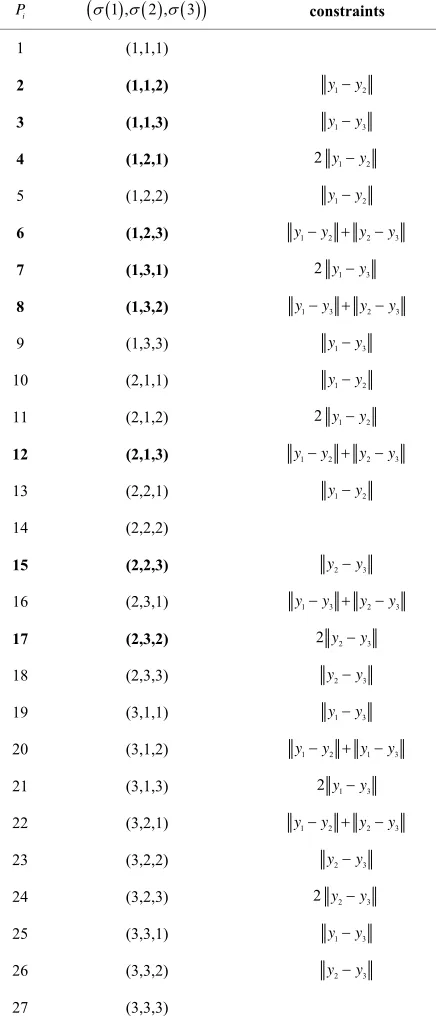
the two previous Sections 3.1 and 3.2 are applied to real data of Dakar Dem Dikk (3D). Recall that 3D (see [20], [21]) is the main public urban transportation company in Dakar. This company manages a fleet of buses with dif- ferent technical characteristics. Some of the buses can operate only in certain roads in the city center and the others can access in all over the network. Buses are park- ed overnight at Ouakam and Thiaroye terminals (see Fig- ure 1).
[image:4.595.57.544.359.704.2]To ensure network coverage, 3D manages its services by using 17 lines, with 11 from Ouakam terminal and 6 from Thiaroye terminal. Each line ensures a certain num-
ber of routes. At present, the total number of routes in the network is 289. First, the most important 18 sites of the network are identified. Thirty (30) permanent terminuses (terminals) and 810 bus stops are used (see Figure 1, where bus stops are not represented due to their size). The map in Figure 1 is obtained by using the software EMME [22]. Table 1 gives the 18 sites, their latitude and longitude.
The data are based on the scenario of 3D; and the input data needed to use the models are the:
total length of the network kilometers;
number of points
= 5902.62
L
k
x (terminals and bus stops) (see Figure 1
latitude and longitude of points
= 18
m );
k
x representing the two terminals and bus stops.
The total distance covered by all the buses from ter- minals to starting points of routes and from end points back to their terminals represents the total length of the network; and we have L = 5902.62 kilometers (for the 18
sites).
The GPS (Global Positioning Sys
nute/60) + (second/3600). Table 1 gives the coordinates of all points.
The numerical experiments are executed:
on a computer: 2 × Intel(R) Core(TM)2 Duo CPU 2.00 GHz, 4.0 Gb of RAM, under UNIX system;
and by the software IPOPT (Interior Point OPTimi- zation) 3.9 stable [23,24], running with linear solver ma27.
For the objective function, we have:
tem) coordinates are calculated with Google map, and then transformed into coordinates on the plane with he formula: degree + (mi-
18
2 2
=1 =1
2
2 2
1 1 2 2 18 18
1 2 18
= min min
= min = min
m
k k k k
k k
x y x y
x y x y x y
with
2
22 1 1 2 2
= = = 1, ,18.
i xi yi xi yi xi yi i
Finally,
18 2 2 18 2
= min j 2 j j
i i i
=1 =1 =1 =1
i j i j
y x y
[image:5.595.59.538.352.734.2]
Table 1. Sc
GPS coordinates
enario of 3D.
Coordinates on the plane
k
x latitude longitude latitude longitude
Ouakam terminal 14˚42'25.79''N 17˚28'43.5
Thiaroye terminal 14˚44'48.49'
2''O 7555555556
.41''O 14.7468027777778 17.3801138888889
9''O 14.7318888888889 17.4441638888889
14˚45'37.04''N 17˚26'16.79''O 14.7602888888889 17.4379972222222
3''O 14.7854777777778 17.3092583333333
1''O 14.6690527777778 17.4412527777778
6''O 14.6529527777778 17.4332944444444
7726111111111 17.3889388888889
Daroukhane 14˚46'53.08''N 17˚22'19.47''O 14.7814111111111 17.3720750000000
1''O 14.7232055555556 17.4586694444444
'O 14.6712611111111 17.4314055555556
Liberte 6 14˚43'42.11''N 14.7283638888889 17.4600888888889
Aeroport 14˚44'44.02''N 17˚29'21.65''O 14.7455611111111 17.4893472222222
Khour 14˚44'59.60''N 17 24'25.10''O 14.749888888 9722222222
Palais1 14 N 17 14.65 8 17.4 44
14.7071638888889 17.478
'N 17˚22'48
Camberene 2 14˚43'54.80''N 17˚26'38.9
PA
Keur Massar 14˚47'7.72''N 17˚18'33.3
Lat Dior 14˚40'8.59''N 17˚26'28.5
Palais2 14˚39'10.63''N 17˚25'59.8
Guediawaye 14˚46'21.40''N 17˚23'20.18''O 14.
Dieuppeul 14˚43'23.54''N 17˚27'31.2
Leclerc 14˚40'16.54''N 17˚25'53.06'
17˚27'36.32''O
ounar ˚ 8889 17.406
˚39'10.63'' ˚25'59.86''O 2952777777 3329444444
Malika 14˚47'37.78''N 17˚20'11.42''O 14.7938277777778 17.3365055555556
Rufisque 14˚42'44.30''N 17˚16'1.66''O 14.7123055555556 17.2671277777778
Ouakam 14˚43'56.98''N 17˚29'35.02''O 14.7324944444444 17.4930611111111
and = 18
j 2 i 2 =1 =1 i jx
is adde e of thetive func
Constr
d to the valu objec-
tion.
aint 1 1 =1
, 0
m
k k
x y yk gives
k
2
1
,
k k
x y y 1 2 3 2
=1
= ,
k k
x y y
Urban t tation networ Thus,
1 2,
y x y
0.
ranspor k of 3D
1, 1 1 2 2 2 3
x y
x x y, 0, i.e.:
And
,
x y
1 2 21 1 1 2 2
2 2 2
2 2 3 2 3 0.
x y x
y x y x y
x x
1 1 1
x y
1 1 1
x y
1 1 2 2
1 2
1
1 =1
m
k k
y L
yk gives2
1 = 1
k
y y L,
e.:
2 2 3
y y y
=1
k k
y
i.
1 1
2 2
1 2 1
2 2 2
2 1 1 2 2
2 2 3 2 3
y y y y y y y y L
with 1 1
4 = 1
y y and y42= y12. ulate the p
We simply m in AM
x, and solve h the AM
form roble PL [25] syn- ta the problem throug PL environ- ment; with a total number of 38 variables for problem . The solution obtained is an optimal one (for each rein the priority is assigned to the minimization
1case) whe
of the distance between xk and yk. The
optimal point within desired toleranc
IPOPT found es; an tain
e follow otal num s 16
d for th k we
an d we ob
th ing results: the t ber of iterations i an e optimal networ opt have
2, ,m 1
=
k k
y x k . The others obtained solutions
1
y, ym and ym1 are given in Ta GPS
and d in
Permut resolutio ed
can gi . The num ems
o solve de ber of p ork.
us, we ints in 3
Now, ermutatio ain
ea of th lem such
at
ble 2 with the co
t
ordinate
he network (see Figure 2
s. The points y1
). m
y are represente
ations make the n more complicat but ve better results ber of sub-probl t
Th
pends on the num choose m= 3 po
oints in the netw D’s network. let us take the p n which is the m id
th
is work. For prob
2 , i= 1, 2,3
i =
i 1
, we have y i y i1 = 0
ar a
-
simil sub-
roblems n:
nd we have 9
. There
fore some constraints are p to solve. An illustratio
1
( ) ( 1 m
k k
y y
) 2 (=1 (2)
=
k
y
y y
The thr sub-prob for
) ( 1) k y k =1
k
(1) (2)
= y y (3)
ee unconstrained lems are obtained
( (1), (2), (3)) with (1) = (2) = (3) , i.e. in the
nts n Table 3.
. y
coor
[image:6.595.56.283.83.391.2]three permutations (1,1,1), (2,2,2) and (3,3,3). All sub-problems constrai are reported i
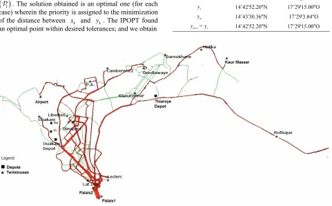
Table 2 1and ym for optimal network Σopt.
GPS dinates
k
y latitude longitude 1
y 14˚42'52.20''N 17˚29'15.00''O
m
y 14˚43'30.36''N 17˚29'3.84''O
=
[image:6.595.59.540.424.722.2]ym1 y1 14˚42'52.20''N 17˚29'15.00''O
Table 3. All constraints with permutations. constraints
i
P
1 , 2 , 3
1 (1,1,1)1 2
y y
2 (1,1,2)
3 (1,1,3) y1y3 4 (1,2,1) 2 y1y2
5 (1,2,2) y1y2
6 (1,2,3) y1y2 y2y3 7 (1,3,1) 2 y1y3 8 (1,3,2) y1y3 y2y3
9 (1,3,3) y1y3
10 (2,1,1) y1y2
11 (2,1,2) 2 y1y2
12 (2,1,3) y1y2 y2y3
13 (2,2,1) y1y2
14
15 (2,2,3)
(2,2,2)
2 3
y y
16 (2,3,1) y1y3 y2y3 17 (2,3,2) 2 y2y3
18 (2,3,3) y2y3
19 (3,1,1) y1y3
20 (3,1,2) y1y2 y1y3
21 (3,1,3) 2y1y3
22 (3,2,1) y1y2 y2y3
23 (3,2,2) y2y3
24 (3,2,3) 2 y2y3
25 (3,3,1) y1y3
26 (3,3,2) y2y3
27 (3,3,3)
It is sufficient to and
ince we ,
only com he quantities
solve P P P P P P P P P1, , , , , , ,2 3 4 5 6 7 11, 14 27= 14= 1
P P P, P13=P10=P5
4
=
P P , P22=P6, P21=P7, 17
=P and P26=P23=P18 16
P
2 16
; s have =P2
15
=P .
5
= 19 9
= = =
P P P P,
8
P P, P20=P12 3 11
, P24
We pute t y1y2 , y1y3
and y2y3 . l sub-problems ,
the jective funct s the same as pr For al
ion i
= 1 , 27
i
P i oblem
,
ob
1 with= 3
m .
3
2 2
=1 =1
2
2 2
1 1 2 2 3 3
1 2 3
= min min
= min = min
m
k k k k
k k
x y x y
x y x y x y
with
1 1
2 2 2 2 1= x1 y1 x1 y1 ,
1 1
2 2 2 2 2= x2 y2 x2 y2
and
1 1
2 2 2 2 3= x3 y3 x3 y3 .
Finally,
and
1 2 2 2 1 2 2 2 1 2 2 21 1 2 2 3 3
1 1 2 2 1 1 2 2 1 1 2 2
1 1 1 1 2 2 2 2 3 3 3 3
= min
2 2 2 2 2 2
y y y y y y
x y x y x y x y x y x y
3 2 2
=1 =1
= j
i i j
x
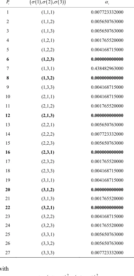
is added to the value of the objec-m computa results, we have obtained the same value for all 10 sub-problems. Thus, permutations do not in he distance constraint on the curve of
tive function.
Fro tional
fluence t k. The
optimal value is = 1170.332935387, for all with problem
i
P
= 1, , 27
i .
For
3 , we consider and the um-be possible is . Recall
that the numbe problems on the nu r of poin networ
po in 3D’s k. Thus, mu
k
k 1,solve o, we c th
n r of
r of su ts n
permutation
b-
2,3
to depends k. Als hoos
for e consid
mbe in the e m= 3
ed per- ints
tation
etwor er
3
sub-pr
1 , 2
ob
we
, have obtained a total of
3
3 = 27 lems P ii
= 1, , 27
to solve, see Ta-ble 4.
In order not to d explanations, we develop only e sub-problem , the rest are left to the reader as an
I lem is obtained for overloa
th 1
exercise.
n 2, the sub-prob 1
P
P
1, 2 , 3 =
1,1,1
, with vectors =
1, 2
i i i
x x x and yi=
y yi1, i2
i= 1, 2,3.For the objective function, we have
3
2 2
= m
1 ( ) ( )
=1 =1
2 2 2
1 (1) 2 (2) 3 (3)
min min
= min
k k k k
k k
x y x y
x y x y x y
2
2 2
1 1 1 2 1 3
1 1 1
1 2 3
= min
= min
x y x y x y
Table 4. Optimal values of αi with different permutations.
i
P
1 , 2 , 3
i1 (1,1,1) 0.007723332000
2 (1,1,2) 0.005650763000
3 (1,1,3) 0.005650763000
(1,2,1) 0.001765520000
5 (1,2,2) 0.004168715000
6 (1,2,3) 0.000000000000
7 (1,3,1) 0.438482963000
8 (1,3,2) 0.000000000000
(1,
2,1,1) 0.004168715000
000
2,2,2) 0 0
(2,2 0.00
0.000000000
(3,1,1)
20
(3,2,2) 0.004168715000
00
25 (3,3,1) 0.00 63000
3,3,2) 0.005650763000
0.007723332000 4
9 3,3) 0.004168715000
10 (
11 (2,1,2) 0.001765520000
12 (2,1,3) 0.000000000000
13 (2,2,1) 0.005650763
14 ( .0077233320 0
15 ,3) 5650763000
16 (2,3,1) 000
17 (2,3,2) 0.001765520000
18 (2,3,3) 0.004168715000
19 0.004168715000
(3,1,2) 0.000000000000
21 (3,1,3) 0.001765520000
22 (3,2,1) 0.000000000000
23
24 (3,2,3) 0.0017655200
56507
26 (
27 (3,3,3)
with
2 21 1 1 2 2
1= x1 y1 x1 y1
,
2 21 1 1 2 2
2= x2 y1 x2 y1
and
2 21 1 1 2 2
3= x3 y1 x3 y1
Finally,
2 2
1 2 1 1 1
1 1 1 1 2
2 2
1 1
= min 3 3 2
2
y y x x x
x x x y
1 1 y and 3 2 2
2 3
3 2 2
=1 =1
= j
i i j
x
is,
i
P i= 1, , 27.
added to the jec-
tiv nction for a roblems The constraint
value of the ob
e fu ll sub-p
1 1 =1 k m k k
y y L
gives
2 1 =k 1 2 2 =1 k
k
y y y y y y3 L
i.e
, .:
1 1
2 2 2
2
1 1
2 2 2
22 3
1 2 1 2 2 3
y y y y y y y y L
e scenar problems
For th io of
2
and
3 , wechoose x1 = Ouak inal, x2 = and
x3 = Leclerc (see ).
We denote by
am term Thiaroye terminal
Table 5
i and
of su * , k i y prob
the opti the op l solution b- lem
spectively.
esults sho the following ms: give the
mal value and
= 1, 2,3
k
, re-
tima Pi
The r w that six sub-proble
6
P , P8, P12, P16, P20, P22 best value
= = 0.0,
. The six sodiffe
=
i
rent,
6,8,12,16, 20 and 22
i re lu- with only The curve
tions a i.e.:
* * * *
,6 ,8 ,12 ,16 ,20 ,22
k k k k k k
y y y* y y y* ,
* ,6= k k
y x .
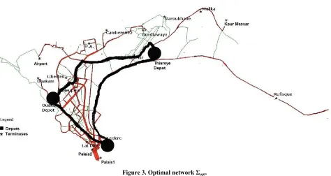
opt
can be described by one of the points
*, k i k
y T x ; see Figure 3 where
1 , 2 , 3
.
The points * h define ates
, k i
y whic opt (with coordin
* , j k i
y j= 1, 2) are tions gi
given in Ta , with ving the be ssible
um) are illustrated in Table 6 and include all per- mutations
ble 6
st po ,6 =
k k
y x . permutations The
(optim solu
i
j i, . the simu
j
According to lations, we determine a set of optimal policy that can describe the optimal network
opt
. Finally: after com we c
parison of the simulated models, an deduce that the model for problem
3optim is It provides the best curve describing the al better.
value opt, obtaine
ective
d with the permutations intro in function.
4. Conclusions
In this paper, we describe applications of mass trans- heory and
n of urban netw
programming problems scribed urban trans- po of 3D applied to these three models. The results have shown that the optimal network is ob- tained with permutations including j
uture works, we will
and make a reformulation that solves a unique prog
duced the obj
portation t develop how to optimize the curve desig ork problems. Using the discrete for- mulations, we give three nonlinear
with continue variables, and have de rtation problem
i
j i, . study an application in
In f 3
network Σopt.
Figure 3. Optim 5. The network Σ with pe
al
Table opt rmutations.
GPS coordinates
instead of solving m
m problems.
. Acknowledgements
5
k
x latitude longitude
We would like to thank all DSI’s (Division Système d’Information) members of 3D for their time and efforts for providing the data, and discussions related to the meaning of the data.
REFERENCES
[1] A. Figalli, “Optimal Transportation and Action-Mini- mizing Measures,” Ph.D. Thesis, Scuola Normale Supe-riore, Pisa, 2007.
[2] G. Buttazzo, E. Oudet and E. Stepanov, “Optimal Trans-portation Problems with Free Dirichlet Regions,” Pro-gress in Non-Linear Differential Equations, Vol. 51, 2002,
pp. 41-65.
[3] G. Buttazzo, A. Pratelli, S. Solimini and E. Stepanov, “Optimal Urbain Networks via Mass Transportation,”
Lecture Notes in Mathematics, Vol. 1961, 2009, pp. 75-
103.
[4] G. Buttazzo, “Three Optimization Problems in Mass Trans- portation Theory,” Nonsmooth Mechanics and Analysis
2 006, pp. 13-23.
[5] E. Oudet, “Some Results in Shape Optimization and
Op-?page=cv/node2
[6] Am matic volving
Inter-faces,” 2, 2003,
p . 1-5
[7] L Amb illi, “S n ‘An n Metric punti uti da D centi delle Scuola, Scuola Normale superiore, Pisa, 2000. 1
x 14˚42'25.79''N 17˚28'43.52''O
2
x 14˚44'48.49''N 17˚22'48.41''O
3
[image:9.595.59.310.459.734.2]x 14˚40'16.54''N 17˚25'53.06''O
Table 6. The optimal solutions with permutations.
GPS coordinates
*
k,i
y
k
y latitude (j = 1) longitude (j = 2)
1,6
y 14˚42'25.79''N 17˚28'43.52''O
14˚44'48.49''N 17˚22'48.41''O (1,2,3) 14˚40'16.54''N 17˚25'53.06''O 14˚42'25.79''N 17˚28'43.52''O 14˚40'16.54''N 17˚25'53.06''O (1,3,2) 14˚44'48.49''N 17˚22'48.41''O 14˚44'48.49''N 17˚22'48.41''O 14˚42'25.79''N 17˚28'43.52''O (2,1,3) 14˚40'16.54''N 17˚25'53.06''O 14˚40'16.54''N 17˚25'53.06''O
14˚42'25.79''N 17˚28'43.52''O (2,3,1)
14˚44'48.49''N 'O
14˚40'1 17˚25'53.06 3,1,2)
14˚ 17˚28'43.52''O
14˚ 17˚25'53.06''O
14˚ 17˚22'48.
14˚42'25.79''N 17˚28'43.52''O
2,6
y
3,6
y
1,8
y
2,8
y
3,8
y
1,12
y
2,12
y
3,12
y
1,16
y
, Vol. 1 , 2
2,16
y
3,16
y timization,” 2002.
http://www-ljk.imag.fr/membres/Edouard.Oudet/index.ph 14˚44'48.49''N 17˚22'48.41''O
1,20
y 17˚22'48.41' p
L. brosio, “Mathe al Aspects of E
Lectures Notes in Ma
2. thematics, Vol. 181 p
. rosio and P. T elect Topics o alysis o Espaces’,” Ap dei Corsi Ten o 2,20
y y
6.54''N ''O (
42'25.79''N
3,20
y1,22
y
40'16.54''N
44'48.49''N 41''O (3,2,1)
2,22
[image:9.595.53.539.462.744.2][8] L. Caffarelli, M. Feldman an n, “Construct-ing Optimal Maps for Monge’s a L mit o ex Co
Mathem , Vol. 1 , pp. 1-26. d i:10. 47-01
d R. J. McCan Transport Prob
sts,” Journal of the American
lem as i f Strictly Conv
atical Society 5, No. 1, 2002 o 1090/S0894-03 -00376-9
[9] L. C. . Gan tial
Methods for ass Transfer P blem f the American Mathematical Soci-ety, Vo , 1999
[10] A. Pra e of O M d
Regular sport sse Transporta-tion Pr . Thesi ale Sup P a, 20 t.sns.
[11] C. Vill Optim ion,” Graduate S dies s, Vol
[12] C. Vill Transp ew,” Springer, Berlin, 2008
[13] V. N. Sudakov the Theory of
eedings of the
, 1976, pp. 1-178.
nsportation and Applications,”
T Prepint, 2006. http://cvgmt.sns.it [16] G. Buttazzo, C. Jimenez and E. Oudet, “An Optimization
Problem for M Congested Dy mics,” SIAM Jo
ort .D. Thesis, Scuola
03.
ol. 2, No. 4, 2003, pp.
outes to a Ter-
Consultants Inc., “EMME User’s Manual,” 2007.
ol. 16, No. 1, Evans and W
the Monge-Kangbo, “Differentorovich M Equations
Nor
[19] ro ,” Memoirs o
l. 137, No. 653 , pp. 1-66.
telli, “Existenc ptimal Transport aps an ity of the Tran
oblems,” Ph.D
Density in Ma
s, Scuola Norm eriore, [20] 631-678. C. B. Djiba, “Optimal Assignment of R is 03. http://cvgm it/
ani, “Topics in al Transportat
tu in Mathematic . 58, 2003.
ani, “Optimal ort, Old and N .
, “Geometric Pr
Dimensional butions,” oblems inProc
vers
I inite Distri
Steklov Institute of Mathematics, Vol. 141
nf [23]
[14] Y. Brenier, “Optimal Tra
Extended Monge-Kantorovich Theory,” Lecture Notes in Mathematics, Vol. 1813, 2003, pp. 91-121.
[15] G. Carlier, C. Jimenez and F. Santambrogio, “Optimal Transportation with Traffic Congestion and Wardrop Equilibria,” CVGM
ass Transportation with
urnal on Control and Optimization
na- , Vol. 48, No. 3, 2009.
[17] F. Santambrogio, “Variational Problems in Transp Theory with Mass Concentration,” Ph
male Superiore, 2006.
[18] A. Brancolini and G. Buttazzo, “Optimal Networks for Mass Transportation Problems,” Preprint Diparttimento di Matematica Universit di Pisa, Pisa, 20
G. Buttazzo and E. Stepanov, “Optimal Transportation Networks as Free Dirichlet Regions for the Monge-Kan- torovich Problem,” Annali della Scuola Normale Superiore di Pisa—Classe di Scienze, V
minal for an Urban Transport Network,” Master of Re- search Engineering Sciences, Cheikh Anta Diop Uni-
ity, ESP Dakar, 2008.
[21] Dakar Dem Dikk, Full Traffic 2008-2009, File Input- Output, 2008. http://www.demdikk.com
[22] INRO
A. Wächter and L. T. Biegler, “Line Search Filter Methods for Nonlinear Programming: Motivation and Global Con- vergence,” SIAM Journal on Optimization, V
2005, pp. 1-31. doi:10.1137/S1052623403426556 [24] A. Wächter and L. T. Biegler, “On the Implementation of
a Primal-Dual Interior Point Filter Line Search Algorithm for Large-Scale Nonlinear Programming,” Mathematical Programming, Vol. 106, No. 1, 2006, pp. 25-57.
doi:10.1007/s10107-004-0559-y