A New Perspective of the Force on a Magnetizable Rod inside a Solenoid

(1)

ISSN Print: 1942-0730

DOI: 10.4236/jemaa.2018.1010013 Oct. 16, 2018 171 Journal of Electromagnetic Analysis and Applications

A New Perspective of the Force on a

Magnetizable Rod inside a Solenoid

José-Luis Jiménez-Ramírez

1*

_{, Ignacio Campos-Flores}

1

_{, José-Antonio-Eduardo Roa-Neri}

2

1_{Departamento de Física, Facultad de Ciencias, Universidad Nacional Autónoma de México, México D. F., México}

2_{Área de Física Teórica y Materia Condensada, División de Ciencias Básicas e Ingeniería, Universidad Autónoma Metropolitana} Unidad Azcapotzalco, México D. F., México

Abstract

We analyze the familiar effect of the pulling of a magnetizable rod by a mag-netic field inside a solenoid. We find that the analogy with the pulling of a di-electric slab by a charged capacitor is not as direct as usually thought. Indeed, there are two possibilities to pursue the analogy, according to the

correspon-dence used, either E→B and D→H, or E→H and D→B. One

of these results in an incorrect sign in the force, while the other gives the cor-rect result. We avoid this ambiguity in the usual energy method applying a momentum balance equation derived from Maxwell’s equations. This method permits the calculation of the force with a volume integration of a force den-sity, or with a surface integration of a stress tensor. An interpretation of our results establishes that the force acts at the interface and has its origin in Maxwell´s magnetic stresses at the medium-vacuum interface. This approach provides new insights and a new perspective of the origin of this force.

Keywords

Force on a Rod in a Solenoid, Magnetostatic Force, Maxwell Momentum Balance Equation

1. Introduction

It is a well-known effect the pulling of a magnetizable rod into a solenoid where a magnetic field is established. There are many practical applications of this ef-fect, like the Bendix mechanism, relays, etc., but how it arises is hardly discussed.

*On sabbatical leave from Departamento de Física, División de Ciencias Básicas e Ingeniería, Un-iversidad Autónoma Metropolitana, Unidad Iztapalapa, Av. San Rafael Atlixco No. 186 Col. Vicen-tina. Apartado postal 21-094, Cd. Mx. 04000.

How to cite this paper: Jiménez-Ramírez, J.-L., Campos-Flores, I. and Roa-Neri, J.-A.-E. (2018) A New Perspective of the Force on a Magnetizable Rod inside a So-lenoid. Journal of Electromagnetic Analysis and Applications, 10, 171-183.

https://doi.org/10.4236/jemaa.2018.1010013

Received: August 16, 2018 Accepted: October 13, 2018 Published: October 16, 2018

http://creativecommons.org/licenses/by/4.0/

(2)

DOI: 10.4236/jemaa.2018.1010013 172 Journal of Electromagnetic Analysis and Applications

This effect is considered analogous to the pulling of a dielectric slab into a paral-lel plate capacitor. The similarity of these effects has been discussed by Boyer [1], and is also discussed in some intermediate texts on electromagnetism [2], [3], [4]. There is, however, a difference about the supposed origin of these effects in the electric and magnetic cases. In the electric case the force acting on the di-electric slab is usually assumed to be caused by the non-uniform fringing field outside the capacitor, [5], [6], [7], [8], [9], while in the magnetic case the fring-ing effects are explicitly neglected [2], [3], and there is no explanation of its ori-gin.

In the electric case, therefore, the force is explained as the action of the non-uniform fringing field on the dipoles of the dielectric slab. We have shown [10] that this force arises rather from the uniform field inside the capacitor transmitted through the Maxwell stresses. In the magnetic case we have a uni-form magnetic field inside the solenoid, which can only align the magnetic di-poles. Therefore, we have the question of how this uniform field can exert a net force on the magnetic dipoles. This is the question we address in the present work. It is rather a conceptual question that we will answer applying the Max-wellian notion of electromagnetic stresses. We use a particular electromagnetic momentum balance equation derived elsewhere [11] from Maxwell’s equations.

We revise first (Section 2) the usual derivation of the magnetic force with energy methods. We find that the usual shortcut of copying the electric case by changing the fields

→

E B and D→H (1)

leads to a wrong sign in the magnetic force. We also discuss the arguments of Landau and Lifshits [12] (Section 3) to show that sometimes the magnetic fields

analogous to E and D are rather H and B, respectively.

Our results point to the tension part of the magnetic stress tensor acting at the interface as the origin of this force (Section 4), explaining in this way how a uni-form magnetic field can exert a net force on magnetizable matter. This consti-tutes a novel point of view that provides insights respect to the electromagnetic force, which is transmitted through stresses, as Faraday and Maxwell anticipated. In Section 5 we present a new force density, Equation (61), from which the magnetic force can be obtained. In Sections 6 and 7 we give theoretical support to this force density showing how it appears in a momentum balance equation. Our approach represents therefore a novel point of view that provides insights respect how the magnetic force arises.

2. Force on a Magnetic Rod inside a Solenoid with Constant

Current

I

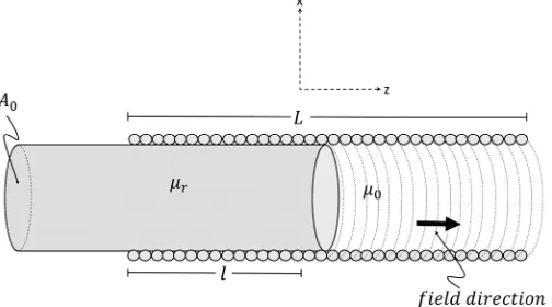
The device is a solenoid of length L, with n turns per unit length, cross area A0

and a constant current I circulating through it. A rod of magnetic material of permeability µr and magnetic susceptibility χm is partially introduced into

(3)

[image:3.595.249.501.75.215.2]

Figure 1. Cylindrical solenoid with a magnetizable rod partially inserted.

Usually this force is derived from the equation

( )

u _I,

=

F ∇ ₍₂₎

where the sub-index I indicates that the process considered occurs with constant current I, hence the positive sign in this equation, and the magnetic energy Um

is given by

all space

1 _{d .}

2 m

U =

_∫

H⋅Β V (3)

(we follow Griffiths [9] and Purcell and Morin [13] and take the field Β as the magnetic field and H as an auxiliary field).

Then, by expressing the H field in terms of the current,

,

nI

=

H (4)

with the constitutive relations

0 r ,

µ µ =

B H (5)

and

1,

m r

χ =µ − ₍₆₎

one can find the known result for the force on the magnetic rod calculating the change in energy in displacing the rod a distance ∆z _[2]_,_[3]_,_[4]_{. This force is}

2

0 0

1 _ˆ.

2µ χmH A =

F k (7)

With this procedure it is irrelevant the fringing magnetic field outside the so-lenoid and what happens at the interface, as noted by Wangsness [2] and Reitz et al.[3].

Now, when a magnetizable material is introduced into a magnetic field, the fields Η and B change, and therefore also the energy changes. If initially there is a vacuum inside the solenoid, the fields are B0 and H0, while after

introducing the magnetizable material maintaining the current constant, the fields are B and Η. Therefore, the change in energy is

(

)

int mat mag 0 _{all space} 0 0

1 _{d .}

2 m

U U U V

(4)

This expression can be transformed in order to have a volume integral only over the volume V' occupied by the material. In the electrostatic case there is al-so a transformation from, [2], [14], [15]

(

)

int matele 1₂ _{all space}d 0 0 ,

U V

∆ =

_∫

E D E D⋅ − ⋅ (9) to

(

)

int matele 1₂ _{all space}d 0 0 ,

U V

∆ =

_∫

E D⋅ −E D⋅ (10)

from which it is deduced that

int matele 1 d₂ _V 0.

U _′ V

∆ = −

_∫

P E⋅ (11)

In order to treat the magnetic case, Jackson [15] and Wangsness [2] propose the correspondence

→

E B, D→H (12)

in the electric case as expressed in Equation (10), obtaining

(

)

int mat mag Jac-Wan 1 d₂ _V 0 0 .

U _′ V

∆ =

_∫

B H⋅ −H B⋅ ₍₁₃₎

Following the steps that in the electric case lead from Equation (10) to Equa-tion (11), they obtain

int mat mag Jac-Wan 1 d₂ _V 0,

U _′ V

∆ =

_∫

M B⋅ (14)

equivalent to

int mat mag Jac-Wan 0

1 _d _.

2 0 V

U µ _′ V

∆ =

_∫

M H⋅ (15)

Jackson [15] and Wangsness [2] call the attention to the difference in sign with respect to the electric case as given in Equation (11). This difference in sign implies a wrong direction in the force. Wangsness [2] obtains the correct result because he does not use result Equation (15) to calculate the force.

It is worth noting that the correct result is obtained if in the electrostatic case, Equation (10), the correspondence E→B and D→H is made, obtaining

int mat mag 0

1 _d _.

2 0 V

U µ _′ V

∆ = −

_∫

M H⋅ (16)

In order to see the consequences of this difference in sign of the change in energy it is convenient to calculate the force with (2) and (15). The equation for the magnetization is

( )

z =χmΘ −

(

l z

)

,

M H (17)

where Θ is Heaviside´s distribution. Then, from Equation (15), the constitu-tive relation (5), (6), and the fact that the H field is constant inside the sole-noid, even inside the magnetic rod, one obtains for the change in energy

(

)

2

int mat mag Jac-Wan 1₂ 0 _V_matd m .

U µ _′ Vχ l z H

(5)

When the gradient is taken using

(

)

(

)

,

z l z δ l z

∂ Θ − = − − ₍₁₉₎

the force results

(

)

2

0 _mat

1 _d _.

2 _V m

F= − µ

_∫

_′ Vχ δ l z H− (20)

After integration the final expression of the force is

2

0 0

1 _ˆ,

2µ χmH A = −

F k (21)

that is, the negative of the correct result (7).

Therefore, the correct result ensues if in the electrostatic result (10) the subs-titution

→

E H and D→B (22)

is made. This points to the fact that in some cases the magnetic fields analogous to the electric fields are

→

E B and D→H (23)

while in others it is the correspondence Equation (22). We have in this respect Stratton’s [16] observation:

“Whatever the analytical advantages of the electrostatic analogy may be, it is well to remember that the physical structure of a field due to stationary distribu-tions of currents differs fundamentally from that of any configuration of electric charges.”

Landau and Liftshitz [12] (L & L in what follows) discuss the problem of elec-tromagnetic fields in matter from a thermodynamic point of view and conclude that in the case of magnetostatics with constant currents the correct analogy is the later, Equation (22). They argue that

1 2 e

u = E D⋅ and 1 ,

2 m

u = H B⋅ (24)

are free energy densities, not total energies, which is fundamental for the under-standing of the interaction of electromagnetic fields and matter. In the next sec-tion we revise their arguments supporting the correspondence Equasec-tion (22).

3. Landau and Lifshitz Thermodynamic Analysis

It is convenient to review with some detail the procedure followed by Landau and Lifshitz [12] with which it is established that in this case the correct analogy is (22).

In the electric case they begin with the work necessary to increase the charge of the system by

δ

q,

.

W q

δ

=

φδ

(25)

(6)

d .

W V

δ =

_∫

E D⋅δ (26)

Then the change in Helmholtz’s free energy, F U TS= − _{, is}

d .

F S T V

δ = − δ +

_∫

E D⋅δ (27)

Note the correspondence

. q

δ

→

δ

D (28)

Now, it is convenient to introduce a thermodynamic potential in which it ap-pears

δ

E instead of

δ

D. This is done by means of a Legendre transformation

* * _.

F =F − ⋅E D (29)

(quantities with asterisk represent densities). The change of this free energy is

* _.

F S T

δ  = − δ − ⋅D Eδ (30)

Therefore, the expressions for the infinitesimal changes in the quantities ex-pressed in terms of the charges and potentials of the conductors are, respectively,

( )

δF T =

∑

kφ δk qk =

∫

φδq Vd , (31)

( )

δ

F T = −

∑

kqk

δφ

k = −

∫

q

δφ

d .V (32)

It is important to note the sign in Equation (32). We have then, besides Equa-tion (27), the correspondence

.

δφ

→

δ

E (33)

In the magnetic case we have an analogous situation, but some care is neces-sary. We have instead of Equation (31) and Equation (32) the equations

( )

δF _T =

_∫

J A⋅δ d ,V (34)

( )

d

T

F V

δ

 = −

_∫

J A⋅

δ

(35)

and L & L point out that in macroscopic electrodynamics the role analogous to the currents is played by the potentials, not by the charges.

These authors [12] observe that

“It is useful to note that in macroscopic electrodynamics the currents (sources of the magnetic field) are mathematical analogues of potentials, not of charges (sources of the electric field). This is seen by comparing Formulaes (31.8) and (31.9) [our Equation (34) and Equation (35)] with the corresponding results for an electric field: [our Equation (31) and Equation (32)].

We observe that the charges and potentials appear in these formulae in the opposite order to the currents and potentials in Formulaes (31.8) and (31.9) [our Equations (34) and (35)].”

In this way the equivalent expressions to (25) and (30) are

d .

W V

δ =

_∫

H B⋅δ (36)

d .

F S T V

δ = − δ −

_∫

H B⋅δ (37)

And for the potential, or free energy, F we have

d .

F S T V

(7)

With this approach they derive straightforwardly the correspondence (22), which implies that the analogy Equation (22) is correct, and therefore the correct expression for the change in energy is Equation (16).

4. Where Does the Force Acts?

The energy methods for calculating the force exerted by a uniform magnetic field inside a solenoid on a magnetizable rod, do not permit establish where and how the force acts. Also, in the analogous electric case of the force exerted on a dielectric slab partially inserted into a parallel plate charged capacitor, the energy method does not allow to establish where and how the force acts. In the electric case, it is said [5], [6], [7], [8], and [9] that it is the non-uniform electrostatic fringing field acting on the dipoles of the dielectric what causes this force. In the magnetic case the fringing non-uniform magnetic field is explicitly neglected.

In order to establish clearly where and how the force arises, it is convenient to apply Maxwell’s magnetic stress tensor. The force in terms of this tensor is, [17]

d ,

σ

=

_∫

⋅

F

_

S T (39)

where T is the magnetic stress tensor.

(

)

1 2

 

=_ − ⋅ _

 

T BH I B H (40) and

σ

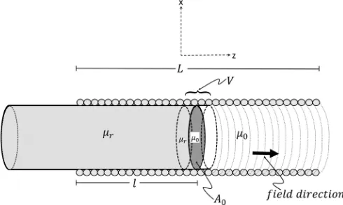
is a closed surface. The relevant surfaces for the calculation are flat sur-face around the intersur-faces formed by a parallels sursur-faces close to the intersur-face, one inside the rod and other in vacuum.

Since for linear magnetic media the constitutive relation (5) implies that B

and H are parallel and in the kˆ direction, the stress tensor becomes

1

ˆ ˆ _,

2

BH 

= _ − _

 

T kk I (41)

where the unit dyad I is

ˆˆ ˆˆ ˆ ˆ_.

= + +

[image:7.595.249.494.544.691.2]

I ii jj kk (42) For the relevant surface we have the differential surface elements (Figure 2)

(8)

medium side

vacuum side

ˆ

d d

ˆ

d d

S S

= − =

S k

S k (43)

With the tensor (41) and the surface elements (43), the expression (39) for the force results

( )

medium vacuum

1 1

ˆ _d ˆ ˆ ˆ _d ˆ ˆ _.

2 2

S BH S BH

σ σ

   

= − ⋅_ − _ − − ⋅_ − _

   

∫

F k kk I k kk I (44)

We have also that

0

ˆ_d_S= ˆ_A_.

∫

k k (45)

Then Equation (44) becomes, using Equation (43),

(

)

_medium

(

)

_vacuum

(

)

_medium

(

)

_vacuum

1 _ˆ 1 _ˆ 1 _ˆ _.

2 2 2

S BH BH  S  BH BH 

= _ + _= _ + _

 

F k k k (46)

Now we take into account the boundary condition

normal medium normal vacuum,

B =B ₍₄₇₎

which with the constitutive relation (5) implies that

normal medium normal vacuum.

rH H

µ = ₍₄₈₎

Therefore

(

)

_medium 1

(

)

_vacuum, r

BH =_µ BH ₍₄₉₎

and then Equation (46) can be written as

(

)

0 vacuum 0

1 _ˆ 1 _{1 ,}

2A BH µ

  

= −   − 

  

 

F k (50)

which can be rewritten as

(

)

(

)

0 vacuum

1 _ˆ _{1 ,}

2A  BH µr 

= _ − _

F k (51)

or in the form

( )

2 0 _vacuum

1 _ˆ _.

2A  H χm

= _ _

F k (52)

This is the correct known result, Equation (7).

We can then conclude that the force acts at the interface magnetic rod-vacuum inside the solenoid and arises from the Maxwell magnetic stress tensor. This “magnetic pressure” was introduced and discussed by Maxwell, thus confirming that the fringing field is irrelevant.

5. The Force Density

As in the electrostatic case, usually we do not deal directly with a force density; this is obtained as a gradient of an energy density and in this way the result Equ-ation (7) is obtained. Now, what is the force density in terms of the fields B or

H and the magnetization M?

(9)

(

)

new′ M = −1₂µ0 0× × ,

f H ∇ M (53)

analogous to the electric force density [15]

(

)

new′ E = −1₂ × × ,

f E ∇ P (54)

from which the known result for the capacitor follows.

In this case the magnetization M depends only on z and is discontinuous at the interface. Since M is in the direction of H, which points in the z direc-tion, we have

0,

×M =

∇ ₍₅₅₎

and therefore

newM 0,

f′ = ₍₅₆₎

showing that we have here a different situation from that in the electrostatic case. However, if we consider the magnetic energy density analogous to that of the electrostatic field,

0

1 2

u′ = − M H⋅ (57)

and calculate f =

( )

∇u _I_{, then}

0

1 _.

2µ

 

= − _ ⋅ _

 

f ∇ M H (58)

With the vector identity for the gradient of a scalar product, the force density results

(

)

(

)

(

)

(

)

0

1 _.

2µ + + +

= _ ⋅ ⋅ × × × × _

f M ∇ H H ∇ M M ∇ H H ∇ M (59)

The last term is zero, as argued above, while the magnetostatic nature of the field and the absence of free currents imply

0

×H=

∇ (60)

leaving only the two first terms; but the field is uniform, so that we are left only with the second term,

(

)

newM = −1₂µ0 ⋅ .

f H ∇ M ₍₆₁₎

This force density is also unusual, expecting rather something like

(

)

new′ M = −1₂µ0 ⋅ ,

f M ∇ H (62)

analogous to the known electrostatic force on a dielectric in a non-uniform elec-trostatic field. In this case, the new force density Equation (61) results

( )

(

)

newM = −1₂µ0H ∂z z .

f M (63)

which is not zero even in the case of a uniform field. Moreover, since

( )

z =χmΘ −

(

l z

)

,

(10)

then from Equation (63) it follows that

(

)

2

newM =1₂µ χ0 0H δ l z− ˆ,

f k (65)

as in the electrostatic case. Integrating this force density over any volume around the interface gives

new vol around interface Md dS z.

=

_∫

F f (66)

Since the volume element is A z0d , where A0 is the cross section of the

magnetizable bar, we have

new 0 vol around interface MA zd ,

=

_∫

F f (67)

then

(

)

2

0 0 0

vol around interface

1 _{ˆ d}

2µ χ H δ l z A z

=

_∫

−

F k (68)

and the force on the magnetic bar of cross section A0 is then

2

0 0 0

1 _ˆ

2µ χ H A ,

=

F k (69)

which is the known result, [2], [3], [4], Equation (7), implying that the adequate force density is

(

)

new 0

1 2

M = − µ ⋅ .

f H ∇ M (70)

We have then, as in the electrostatic case, a new force density that gives the correct result. The electrostatic and magnetostatic cases seem very similar, but the force densities differ in both cases. This motivates looking for a more general momentum balance equation that includes, in the magnetic case, the force den-sity Equation (61). In the next section we search for such balance equation.

6. Momentum Balance Equation for Magnetic Materials

The question is if the momentum balance equation [17], [18]

(

)

(

)

(

)

( )

(

)

( )

1 2 1 2

t

ρ

 

⋅_ + − ⋅ + ⋅ _− ∂ ×

 

= + × + _ ⋅ − ⋅ + ⋅ − ⋅ _

DE BH I D E B H D B

E J B E D D E H B B H

∇

∇ ∇ ∇ ∇

(71)

includes the new force density Equation (61). The magnetostatic force density is different from the electrostatic force density, but we can proceed as in the elec-trostatic case.

If only magnetostaic fields are involved, and there are not free charges and currents, Equation (71) transforms in

(

)

(

)

( )

1 1 _.

2 2

 

⋅ − ⋅ = _ ⋅ − ⋅ _

BH I B H  H B B H

∇ ∇ ∇ ₍₇₂₎

The constitutive relation

(

)

0

µ

= +

(11)

and the dyadic identity

( )

∇a b a⋅ = ×

(

∇× +b

) (

a⋅∇

)

b₍₇₄₎

permits to write the right member of Equation (72) in the form

(

)

(

)

(

) (

)

(

) (

)

1 2 1 _. 2 ⋅ − ⋅     = _ × × + ⋅ − × × − ⋅ _

H M M H

M H M H H M H M

∇ ∇

∇ ∇ ∇ ∇ (75)

Since we are dealing with the magnetostatic case without free current densi-ties, we have

0,

×H=

∇ (76)

and from Equation (55),

0.

×M =

∇ (77)

Furthermore, the magnetic field and magnetization are in the z direction, so

(

M⋅∇

)

H=0,₍₇₈₎

remaining

(

)

(

)

(

)

0 0

1 1

2µ ∇H M⋅ − ∇M H⋅ =−2µ H⋅∇ M (79)

which is the result we were looking for and agrees with the force density Equa-tion (61). Then we have

(

)

(

)

( )

(

)

0 new 1 1 2 2 1 _.

2µ M

 

⋅ − ⋅ = _ ⋅ − ⋅ _

 

= ⋅ =

BH I B H H B B H

H M f

∇ ∇ ∇

∇ −

(80)

7. General Balance Equation

We can conclude from the above results that the balance equation Equation (71) implicitly contains the new electric and magnetic force densities, and it is conve-nient therefore to rewrite it in a form where these force densities appear expli-citly. This can be achieved gathering the result of Equation (79) and the analog-ous one for the electric part [10], with which the balance Equation (71), can be written in the form

(

)

(

)

(

)

( )

(

)

( )

(

) (

)

(

) (

)

0 1 2 1 2 1 _. 2 t ρ µ   ⋅_ + − ⋅ + ⋅ _− ∂ ×   = + × + _ ⋅ − ⋅ + ⋅ − ⋅ _ + _ × × + ⋅ − × × − ⋅ _

DE BH I D E B H D B

E J B E D D E H B B H

M H M H H M H M

∇

∇ ∇ ∇ ∇

(81)

(12)

8. Conclusions

We have calculated, in a novel and insightful way that allows a physical explana-tion, the well-known force that arises when a magnetizable rod is partially in-troduced into the magnetic field of a solenoid. Our approach is an alternative to the usual calculation with the gradient of an energy. The usual calculation does not give any insight about where the force acts and how it arises, while our me-thod does give such insights. This novel calculation is based on the volume inte-gration of a force density and the surface inteinte-gration of a magnetic stress tensor. Though the force density may seem unfamiliar, it is part of a momentum bal-ance equation derived directly from the macroscopic Maxwell equations. Indeed, these balance equations contain many force densities, for example the Helmholtz force density [11], with which this magnetic force can also be calculated. This method leads to results that indicate that this force is exerted at the rod-vacuum interface, where the magnetic field is uniform, and has its origin in Maxwell’s magnetic stresses.

We also analyze the analogy with the electric case, used sometimes to calculate the force as a gradient of a magnetic energy. The proposed analogy consists in substituting in the electric case E with B and D with H. The analysis of this familiar effect shows that the classical theory of electromagnetism still con-tains interesting conceptual aspects that deserve attention.

Conflicts of Interest

The authors declare no conflicts of interest regarding the publication of this pa-per.

References

[1] Boyer, T.H. (2001) Electric and Magnetic Forces and Energies for a Parallel-Plate Capacitor and a Flattened, Slip-Joint Solenoid. American Journal of Physics, 69, 1277-1279. https://doi.org/10.1119/1.1407255

[2] Wangsness, R.K. (1986) Electromagnetic Theory. 2nd Edition, John Wiley and Sons, New York.

[3] Reitz, J.R., Milford, F.J. and Christy, R.W. (1993) Foundations of Electromagnetic Theory. 4th Edition, Addison-Wesley, Reading.

[4] Nayfeh, M.H. and Brussel, M.K. (2015) Electricity and Magnetism. Dover, Mineola. [5] Margulies, S. (1984) Force on a Dielectric Slab Inserted into a Parallel-Plate

Capa-citor. American Journal of Physics, 52, 515-518.https://doi.org/10.1119/1.13861

[6] Utreras-Diaz, C. (1988) Dielectric Slab in a Parallel-Plate Condenser. American Journal of Physics, 56, 700-701. https://doi.org/10.1119/1.15504

[7] Naini, A. and Green, M. (1997) Fringing Fields in a Parallel-Plate Capacitor. Amer-ican Journal of Physics, 45, 877-879. https://doi.org/10.1119/1.11075

[8] Dietz, E.R. (2004) Force on a Dielectric Slab: Fringing Field Approach. American Journal of Physics, 72, 1499-1500. https://doi.org/10.1119/1.1764563

(13)

DOI: 10.4236/jemaa.2018.1010013 183 Journal of Electromagnetic Analysis and Applications [10] Campos-Flores, I., Jiménez-Ramírez, J.-L. and Roa-Neri, J.-A.-E. (2018) How Does Arise the Force on a Dielectric Slab in a Parallel Plate Capacitor? Journal of Elec-tromagnetic Analysis and Applications, 10, 131-142.

https://doi.org/10.4236/jemaa.2018.107010

[11] Campos, I., Jiménez, J.L. and López-Mariño, M.A. (2012) Electromagnetic Mo-mentum Balance Equation and the Force Density in Material Media. Revista Brasi-leira de Ensino de Fisica, 34, 2303.

[12] Landau, L.D., Lifshitz, E.M. and Pitaevskii, L.P. (1984) Electrodynamics of Conti-nuous Media, Vol. 8 Course If Theoretical Physics. 2nd Edition, Pergamon, Oxford. [13] Purcell, E.M. and Morin, D.J. (2013) Electricity and Magnetism. 3rd Edition,

Cam-bridge, New York.

[14] Becker, R. (1982) Electromagnetic Field and Interactions. Dover, Mineola.

[15] Jackson, J.D. (1998) Classical Electrodynamics 3rd Edition, Wiley and Sons, New York.

[16] Stratton, J.A. (1941) Electromagnetic Theory. McGraw-Hill, New York.

[17] Panofsky, W.K.H. and Phillips, M. (1962)Classical Electricity and Magnetism. 2nd Edition, Addison-Wesley, Reading.

[18] Jiménez, J.L., Campos, I. and López-Mariño, M.A. (2011) A New Perspective of the Abraham-Minkowski Controversy.The European Physical Journal—Plus, 126, 50.