Abstract— During the element creation procedure of initial mesh generation using the standard advancing front technique (SAFT) , there is a possibility where a conflict of undecided element occurs which do not follow the normal cases. We proposed a direct approach to tackle this kind of problem by extending the two normal cases in SAFT to the total number of five cases of consideration during the element creation procedure in initial mesh generation. The approach is called as Enhanced Advancing Front Technique-1 (EAFT-1). The aim of the work is to improve the SAFT in order to tackle directly such problem of sudden invalid triangular element without having to re-order back the Front list and without erasing the existing element in the initial mesh generation. A simulation of this approach has been done and the quality of the mesh is examined using a number of defined measurements in Gambit software. The resulted mesh is applied for modeling the radiation heat transfer problem using Discrete Ordinate method.
Index Terms— Initial mesh, Enhanced Advancing Front
Technique, extended cases and radiation.
I. INTRODUCTION
TRUCTURED or unstructured triangular mesh formation is an important step for approximating solutions to boundary value problems. Recently, unstructured grid has been predominant because of its ability of modeling complex geometries, besides its natural environment for adaptivity [1]-[3]. Triangular element is chosen in this work since it is reported that these type of element are the most flexible for automatic mesh generation particularly when mesh grading is required [1], [2]. Among the famous method of generating unstructured mesh is Delaunay triangulation and Advancing front technique (AFT). The AFT is guaranteed to preserves boundary integrity as well as it has the capacity to create triangular elements with high aspect ratio in boundary-layer region [2]. In the present paper, we extend the work done in [2] and the issue raised in [4] by illustrating two different conditions
Manuscript received Jan 13, 2011; revised Feb 5, 2011. This work was supported by Ministry of Higher Education, Malaysia under SLAB scholarship.
Z. Abal Abas is now with Department of Mathematics, Faculty of Science, Universiti Teknologi Malaysia, 81310 Skudai, Johor, Malaysia, currently on study leave from Universiti Teknikal Malaysia Melaka. (e-mail: {[email protected]).
S. Salleh is with the Department of Mathematics, Faculty of Science, Universiti Teknologi Malaysia, 81310 Skudai, Johor, Malaysia. (email:
of undecided element creation during the iteration, regarded as conflict during element creation procedure using the Standard Advancing Front Technique (SAFT) which will be described in detail in section II. A brief concept of SAFT and numerical method is described in section III. We present our direct approach of encountering this specific problem by incorporating the five extended cases of consideration during the element creation procedure. The approach is called Enhanced Advancing Front Techniques-1 (EAFT-1) where each of the cases will be explained in Section IV. At the end of the paper, we apply the unstructured mesh for modeling the radiative heat transfer problem using Discrete Ordinate method for a simple two dimensional domain.
II. PROBLEM STATEMENT
In general, the following cases are possible during the procedure of element creation:
(1)A new node (ideal point) is created and been selected as a vertex to form the new triangle element where this new node satisfies certain condition listed in the SAFT.
(2)The already existing front node and active edges are selected to form the new triangle element where this existing node satisfies certain condition listed in the SAFT.
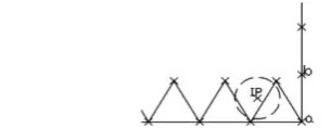
However, there are also conditions which do not belong to any of the above cases. This issue has been raised in [4] where an efficient mesh generation algorithm should be able to tackle such problem when neither the normal case listed above occurs during the element creation. Before illustrating the problem in detail, a few terms need to be defined. We denote an edge as (a,b) which means that the edge is formed by node a and node b. The current selected edges being considered is called as base edge. Front is a list or a set of active edges which is currently available for element triangulation. It must be noted that all the edges belong to the current Front will be considered as active edges while edges that had been drop from the current Front list will be considered as passive edges. At the same time, any nodes which compose the active edges in the current position of the Front list are also known as active node. In the creation of the triangular element, once base edge has been identified, the position of ideal point (IP) on the perpendicular bisector of the base edge is computed in such a way that an equilateral triangle is formed with IP as vertex.
Enhanced Advancing Front Technique with
Extension Cases for Initial Triangular Mesh
Generation
Z. Abal Abas and S. Salleh
Figure 1 illustrates the first condition that does not belong to neither of the normal case. The boundary curve has been discretised into a set of boundary edges where edge (7,8) is a part of the boundary. The procedure of the triangular element creation is conducted smoothly as outlined in the SAFT for the first six elements but when it comes to create the next triangular element, with (7,9) as the base edge, the problem occur when the IP constructed as in Figure 1 is out of the boundary curve and at the same time there is no active node lie within the circle which is appropriate to replace the IP. Appropriate here means the node needs to be inside the boundary as well as the node do not lies within other existing triangular element.
Another condition that might occur in which we classified as the second problem is illustrated in Figure 2 where the base edge being considered is (a,b). There is also a possibility that the IP created is still inside the boundary, but it is too close to the existing element, and one cannot connect the base edge directly to the IP because the side of the new element will intersect the existing side of the triangle element. Furthermore, no active nodes which can replace the IP appropriately lie within the circle. These second condition also leads to conflicts or undecided element creation procedure during the element creation.
According to the algorithm of SAFT in [2], if these happen, one needs to re-order the Front and take the second shortest active edge and repeat the triangulation process again. At some later stage, the same condition may occur and again, one needs to re-order the Front again and select the next active edge. Imagine if we have thousand of edges in a bigger computational domain, this procedure might be complicated and may take longer time to complete the task. Other author in [4] suggests that one might consider to erase a few existing elements if this problem occurs.
Therefore, this scenario shows that the algorithm is not sufficient to cover all conditions, hence an improvement need to be done to tackle the problem directly. Our work focus on how to improve the algorithm of SAFT in order to tackle such problem describe above directly without having to re-order back the Front list and without erasing the existing element in the initial mesh generation. The approach involves studying all types of entities or objects that fall into the circle for further consideration so that the triangular
III. STANDARD ADVANCING FRONT TECHNIQUE AND THE NUMERICAL METHOD
A. The general basic step of standard Advancing Front Technique with background grid
The following basic steps of SAFT in this section are based on [2]. The boundary curves are discretized by dividing the boundary curves into straight line segments and hence, nodes are placed on each of the segment. The main approach of controlling the grid in terms of size and shape of the triangular element involves the definition of the required grid-cell characteristic through background grid generation [1]-[7]. The grid-cell characteristics or known as grid cell parameters are the size parameter
, the stretching s and finally the orientation of the cells. These parameters are required to be defined at each node forming the background grid.Grid cell parameters for all nodes in the Front are interpolated using the value defined at the background grid. The edge with shortest length lin the Front is selected as a departure zone, in order to create the triangular element. In order to obtain
for the next step of calculation, the interpolated values of
corresponding to the two nodes of the edges is averaging. The position of IP on the perpendicular bisector of the side is computed and the empirical formula is used to obtain the radius, r. A circle with centre at IP is constructed with the following empirical formula for the radius, r0 8. *, where
0 55 0 55
0 55 2 0
2 0 2 0
. * l; . * l
; . * l . * l
. * l; . * l
(1)
Active nodes that lie within the circle are searched (if any) and their distances from IP are listed. The best candidate for the third vertex of the triangular element would be the closest one to the IP. The equilateral triangle will be formed if there are no such active nodes lies within the circle. However, the validity of the IP becoming the vertex must be check in which it need to satisfy the following conditions:
(1)The coordinate of IP do not lie inside another existing triangular element.
(2)There is no intersection between the side of the new triangular element and any existing sides of the active front.
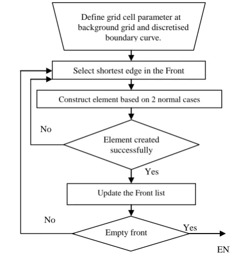
[image:2.595.122.217.61.128.2]Generally, in a ‘marching’ process, the Front moved into the interior of the domain, in which new nodes and edges are created and at the same time old related edges are deleted from the Front list in order to produce triangular element. The new triangular element is constructed by two nodes of a segment of a Front and another node either a newly created or already been existed in the Front. The Front will be updated every time an element is constructed. If the above step of creating the triangular element failed, then one needs to re-order the Front and then select the second shortest active edges as the departure zone for element creation procedure. This process will be continued until there are no Fig. 1. Edge (7,9) as the base edge. The IP is out of the boundary and
no point lie within the circle
[image:2.595.65.218.466.525.2]longer active edges in the Front or the whole computational domain has been triangulated completely. The general scheme for SAFT is illustrated in Figure 3.
B. The concept of radiation and Discrete Ordinate method
Radiation will be emitted more at higher temperature materials. Emissive power Eis a rate of heat flow per unit surface area emitted by a radiating surface. For a black body emissive power, Eb is given by
4 b
E T (2) Where 5 67 10. 8is Stefan-Boltzmann’s constant and
Tis absolute temperature. The intensity Iis the rate of heat flow received per unit area perpendicular to the rays and per unit solid angle. The formula for intensity of the black body,
b
I is
4 b b
I E / T / (3) Equation (3) is used to compute the emitted radiation intensity from the surfaces and fluids.
When combustion occurs, there exist large amount of carbon dioxide and water vapor where these combustion products are both strong absorbers/emitters in the infrared part of the spectrum and this fluid is termed as participating medium [8], [9]. The interaction between participating fluid medium and radiation can be measured in terms of absorption coefficient and its scattering coefficientswhere the sum of these two properties is called extinction coefficient s [9].
The general relationship that governs the changes in radiation intensity at a point along a radiation ray due to emission, absorption and non-scattering in a fluid medium is as follows [10]
b
dI
I I
ds
r,s
r r,s (4)
I r,s is the intensity of radiation at location indicated by position vector r, in direction s. The first and second terms in the right-hand side equation are the emitted intensity and the absorbed intensity respectively. Equation (4) is integrated over each triangular element in the mesh obtained. It is also subject to the boundary condition as follows [10]
i2
1
dΩ 2
b
I I I
w w w i i
r ,s r r ,s n.s (5)
w
r is a position vector for a point on a diffusively emitting and reflecting opaque surface and is surface emissivity.
Iis incident intensity and nis outward surface normal. Using Discrete Ordinate method, equation (4) is solved for a set of nvarious directions si, i1 2, ,...n. A numerical
quadrature replaces the integral over direction, or [10]
4
n i i i
f ( s )d w f ( s )
(6) Where wi is the quadrature weight associated with direction
i
s . Therefore, the approximation of equation (4) is done by a set of nequations [10],
b
dI
I I
ds
i
i
r,s
r r,s (7) With i1 2, ,...nsubject to the boundary conditions [10]
1
1 n
b j
j
I I w I
ww i w w w j j
r
r ,s r r r ,s n.s
(8) IV. THE EAFT-1 WITH THE EXTENSION CASES Our contribution in this paper is to introduce five extended cases which will be used as a guidance to decide the element creation directly. The first two cases are the normal cases as in SAFT while the third, fourth and fifth cases are newly created one. These direct approach involved in the consideration of triangular element creation procedure depends on the condition of objects lie within the circle or at the circum circle. The objects here mean any active nodes or active edges. This is where the construction of the triangular element will be based on.
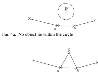
Case 1:
The first case (Case 1) is the simplest one. Let say the current base edge being considered is (a,b), as shown in Figure 4a. A circle at centre IP with radius following the empirical rule is constructed. If there is no object lying within the circle, the IP will turn out to be the third vertex for the triangular element construction. The base edge will be the side of the triangle. The new second and third sides will be (a,c) and (a,b). Since all three sides have equal length, the triangular element formed will be an equilateral triangle element as illustrated in Figure 4b.
Fig. 3. The general scheme of SAFT No
No
Yes
END Yes
Construct element based on 2 normal cases
Update the Front list Define grid cell parameter at background grid and discretised
boundary curve.
Empty front
Select shortest edge in the Front
[image:3.595.55.281.106.357.2]Case 2:
Let say the base edge being considered is (a,b) as shown in Figure 5a to describe the construction of a triangular element based on Case 2. A circle at center IP with radius following the empirical rule is constructed again. There are two types of objects that lie within the circle. First is node d and the second type of object is two active edges intersected with the circle which are edge (c,d) and edge (d,e). Among nodes and edges, this category of extension cases gives priority to nodes when it comes to the selection if both objects occur simultaneously within the circle. If there are multiple active nodes in the circle, calculate all the distance of every active node to the IP. The node which is closest one to IP is selected as the third vertex for triangular element. As illustrated in Figure 5b, node d is selected as the vertex, therefore, a triangular element is constructed with edge (a,b), edge (a,d) and edge (d,b) as the three sides.
Case 3:
At the same time, there is another triangular element being constructed automatically since the three edges are connected to themselves. This condition belongs to Case 3. As illustrated in Figure 5b, a triangular element is constructed automatically when edge (b,d) is formed. The three edges (b,c), (c,d) and (b,d) are connected to themselves, and they become the sides of the second triangular element.
Case 4:
Figures 6a and 6b show the construction of triangulation element following the fourth case (Case 4). Let say the base edge being considered is (a,b) where a circle with radius
constructed. Based on the figure, it can be seen that the only object involved is an active edge which is intersected with the circle. The active edge intersected with the circle is (b,c) as illustrated in Figure 6a. The intersection point of the circum circle with the active edge (b,c) has been marked as points p1 and p2. Based on the algorithm of EAFT, we need to determine the length between the intersection points. In other words, if referring to Figure 6a, we need to determine the length between point p1 and point p2. If the length is less than the radius of the circle, therefore, the intersected active edge is disregarded. Instead, the IP will become the third vertex of the triangular element. Based on Figure 6b, the IP has become node d in which a triangle element is formed with edges (a,b), (a,d) and (b,d) as the three sides of the triangular element.
Case 5:
[image:4.595.55.227.55.189.2]Slightly different from Case 4, if the length between the intersection point p1 and p2 is more than the length of the radius, the active edge intersected with the circle will be considered in which the node of the active edge will be selected as the third vertex. In other words, referring to Figure 7a, since the length of point p1 and point p2 is more than the length of the radius, therefore, node c, which is the node associated with active edge (b,c) will be the vertex to form triangle element as illustrated in Figure 7b. This condition belongs to Case 5. However, if there are multiple edges intersected with the circle and they are all satisfying the condition of Case 5, therefore, the associated node which is the closest to IP will be selected as the third vertex. Fig. 4a. No object lie within the circle
Fig. 4b. An equilateral triangle is constructed
Fig. 5a. Two types of object lie within the circle which are active nodes and edges
Fig. 5b. Node d is selected as the third vertex for triangular element
Fig. 6a. An active edge intersected with the circle
Fig. 6b. The IP become the new active node for triangular element
Fig. 7a. The intersected active edge is (b,c). The length of intersection point p1 and p2 with the circle is more than the length of radius
[image:4.595.312.481.240.389.2]The general scheme of EAFT-1is demonstrated as in Figure 8. It must be noted that most of the basic steps in EAFT-1 is still following the SAFT except that the construction of the element is now based on five extended cases.
V. RESULTS
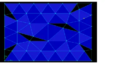
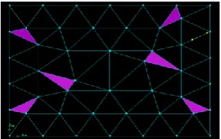
Our approach is applied at a rectangular computational domain as illustrated in Figure 9 with its boundary segment discretized into a set of boundary edges. We use the default value for the size parameter which is five percent from the length of the diagonal of the background grid. The grid generation parameters on the background grid are specified to be
0 56. and s1 at each point of the background grid. The result of initial unstructured mesh with EAFT-1 is illustrated in Figure 10. No re-order Front or erasing a few existing element are needed during the element creation procedure since our extension cases offer a direct approach of deciding element creation when the problem describe insection II occur. The total number of element generated using our approach is 72 and each of the triangular elements has been numbered from 1 to 72.
In order to examine the quality of the mesh, the EquiSize Skew, QEVS which is the measure of skewness is used where it is defined as [11]
eq
EVS
eq
S S
Q
S
(9)
In the above equation, S is the area of the mesh elements, eq
S is the maximum area of equilateral triangle the circumscribing radius of which is identical to that of the mesh element. The value of the examined quality based on this equation provided by [11] is in the range of 0QEAS 1 where QEVS 0 if the element is equilateral triangle and QEVS 1if the triangular element is degenerate (poorly shape). It must be noted that generally, high-quality meshes poses average value of QEVS 0 1. for two dimensional domain [11]. Figure 11a-11c illustrate the corresponding triangular element in the mesh with the range of the quality examined. It can be seen that 83.33% of the elements are in the range of 0QEVS 0 1. which can be considered as a high quality meshes. Therefore, the triangular elements generated using our approach of extending the normal cases to five cases in the standard AFT for element generation procedure prove to work well when there is not normal conditions occur as described in section II.
In order to prove that the triangular mesh work well and is appropriate for computational analysis, the governing equation of radiative heat transfer has been incorporated with the mesh. Using FLUENT version 6.0, simulation had been conducted to solve the radiative heat transfer by using the Discrete Ordinate Methods. Since this is a conceptual model, we imposed the value of the wall temperature (K) so that it can be used as boundary values in the calculation. The simulation is conducted until convergence is reached. Figure 12 shows the flue gas temperature distribution contours between the walls respectively. As shown in the simulation result, the temperature distribution of the flue gas is non-uniform, which will further influence the heat transfer between the walls.
Fig. 9. Rectangular computational domain with a set of boundary edges
Fig. 8. The general scheme of Enhanced Advancing Front Technique -1.
No
Yes END Construct element based on 5 cases
Update the Front list Define grid cell parameter at background grid and discretised
boundary curve.
Empty front
Select shortest edge in the Front
[image:5.595.57.281.119.309.2]Fig. 11a. Element with quality 0QEVS0 1.
[image:5.595.54.278.529.761.2] [image:5.595.345.539.618.720.2]VI. CONCLUSION
In the present work of initial unstructured triangular mesh generation using EAFT-1, the algorithm still uses SAFT method of specifying the grid cell parameter at the background mesh in order to control the mesh size as well as still using the empirical rule to construct the circle for element consideration. The only different is that we proposed the normal case in the SAFT to be extended to five cases in order to encounter the problem of conflict or undecided element creation during the mesh generation procedure. Our EAFT-1 approach of incorporating the extended cases of element creation is able to tackle the problem of element creation directly by considering the entities that lie within the circle constructed. The examined results of initial mesh proved that the approach is able to produce high quality meshes. The simulation results obtained from the FLUENT also support our findings in EAFT-1 for effectively approximating the radiation intensity and temperature values in the two dimensional domain.
ACKNOWLEDGMENT
The authors thanks the Ministry of Higher Education, Malaysia and Universiti Teknikal Malaysia Melaka (UTeM) for sponsoring the research work
REFERENCES
[1] P. R. M. Lyra and D. K. Carvalho, "A computational methodology for automatic two-dimensional anisotropic mesh generation and adaptation," Journal of the Brazilian Society of Mechanical Sciences
and Engineering, vol. 28, 2006, pp. 399-412.
[2] M. Farrashkhalvat and J. P. Miles, Basic structured grid generation
with an introduction to unstructured grid generation: Butterworth
Heinemann, 2003, ch.8.
[3] R. Lohner, "Progress in Grid Generation via the Advancing Front Technique," Engineering with Computers, 1996, pp. 186-210. [4] N. Kovac, S. Gotovac, and D. Poljak, "A New Front Updating
Solution Applied to Some Engineering Problems," Archives of
Computational Methods in Engineering, vol. 9, 2002, pp. 43-75.
[5] J. Zhu, T. Blacker, and R. Smith, "Background overlay grid size functions," in Proceedings of the 11th international meshing
roundtable, 2002, pp. 65–7.
[6] E. Seveno, "Towards an adaptive advancing front method," in 6th
International Meshing Roundtable, 1997, pp. 349–362.
[7] J. Peraire, J. Peiro, and K. Morgan, "Advancing front grid generation," in Handbook of Grid Generation, N. P. Weatherill, B. K. Soni, and J. F. Thompson, Eds.: CRC Press LLC, 1999.
[8] G. Stefanidis, B. Merci, G. Heynderickx, and G. Marin, "Gray/nongray gas radiation modeling in steam cracker CFD calculations," AIChE Journal, vol. 53, 2007, pp. 1658–1669. [9] H. K. Versteeg and W. Malalasekera, An Introduction to
Computational Fluid Dynamics. England: Pearson Education, 2007,
ch. 13.
[10] M. F. Modest, Radiative Heat Transfer, 2 ed.: Academic Press, 2003. [11] "Gambit 2.3 Documentation - Gambit User Guide." vol. 2010:
FLUENT Incorporated.
Zuraida Abal Abas was born in Perak, Malaysia in 1981. She received the BSc in Industrial Mathematics with first class honors from Universiti Teknologi Malaysia, Malaysia in 2002 and MSc in Operational Research from London School of Economics, UK in 2003. Her current research interests include mesh generation, numerical methods and operational research techniques.
Shaharuddin Salleh received the BA in Mathematics from California State University, MSc. in Mathematics from Portland State University, Oregon and Ph.D in Computational Mathematics from UTM. He is currently a Professor at Faculty of Science, Universiti Teknologi Malaysia. His current research interests include numerical modelings and simulations, graph theoretical applications, mobile computing and parallel algorithms. His has written four books which include three at the international level. There are also 65 technical papers in various journals and conferences at the national and international levels.
Fig. 11b. Element with quality 0 2. QEVS0 3.
Fig. 11c. Element with quality 0 4. QEVS0 5.
[image:6.595.87.243.188.286.2] [image:6.595.48.280.319.463.2]