Fuzzy Regulation for the Intelligent Control of
Switching-Mode Buck Power-Electronic Converter
Using Genetic Algorithm-Based Tuning
Anas N. Al-Rabadi, Mahmoud A. Barghash, and Osama M. Abuzeid
Abstract − This article introduces the method of intelligent regulation to control the Buck power-electronic converter using a newly developed small-signal model of the pulse width modulation switch. The implemented method uses a fuzzy-PID controller that is tuned using the global search method of genetic algorithm. The experimental simulation results show that the used intelligent hierarchical regulation method using the GA-tuned fuzzy-PID controller, for the utilized new PWM small-signal model, produces the desired system response for performance enhancement of the electronic switching-mode Buck converter despite the occurrence of noise with comparatively high amplitudes.
Index Terms − Fuzzy logic, genetic algorithms, intelligent control, power-electronic Buck converter, switching-mode power supply.
1. INTRODUCTION
In recent years, small-signal modeling of dynamic behaviors of the open loop power converters has received notable amount of attention, due to the fact that these models are the basis to extract accurate transfer functions which are essential in the feedback control design [7, 31]. They are used to design reliable high performance regulators, by enclosing the open loop DC-to-DC power converters in a feedback loop, to keep the performance of the system as close as possible to the desired operating conditions. The direct purpose of this feedback loop is to counteract the outside noise in the (a) source voltages, (b) duty ratio (the output pulses of the pulse width modulator (PWM)), and (c) load current, in order to regulate the output voltage [7, 31].
The utilized power converters generally operate in (a) Continuous Conduction Mode (CCM) or (b) Discontinuous Conduction Mode (DCM) [7, 31]. The CCM mode is desirable, as the output ripple of the DC-to-DC power converter is very small compared to the DC steady state output. A linearized small-signal model is constructed to examine the dynamic behaviors of the converter, due to the fact that noise is of small signal variations.
This research was performed with the support from the Dean of Academic Research (DAR) at The University of Jordan under grant number (733).
A. N. Al-Rabadi (Corresponding Author) is currently with the Computer Engineering Department at The University of Jordan, Amman-11942-Jordan; phone: +962 79 6445364; e-mail: [email protected]. M. A. Barghash is currently with the Industrial Engineering Department at The University of Jordan; e-mail: [email protected].
O. M. Abuzeid is currently with the Mechanical Engineering Department at The University of Jordan; e-mail: [email protected].
Through this small-signal model, the necessary open-loop transfer functions can be determined and plotted using Bode plots. This is needed in order to use compensation to the pulse width modulation (PWM) power converters, to meet the desired nominal operating conditions, through the application of various control methods. These control methods can incorporate the approaches of: (a) frequency analysis in the classical control theory [32, 77], (b) time analysis in the modern control theory [32, 77], (c) both frequency analysis and time analysis domains in the post modern (digital and robust) control theory [77], and (d) soft computing (e.g., fuzzy logic, neural networks, and genetic algorithms) in the intelligent control methodology [2-4, 8, 10, 13-15, 100]. These control methods can be applied to the models of power converters that usually work with only one specific control scheme, which is pulse width modulation (PWM) through either duty-ratio control or current programming control [31]. In this article, the duty-ratio control is used, in which the switch ON-time is controlled externally by comparing a saw tooth ramp with the controller voltage [31].
Various modeling approaches of the PWM power converters already exist. These approaches can be separated into three main categories. The first modeling category aims towards modeling the whole PWM converters. Examples for this category are (a) volt-second and current-second (charge) balance approach, and (b) state-space averaging approach [7, 31]. These approaches suffer from inaccurate results in the high-frequency range. The second modeling category aims more specifically towards modeling what is called the converter cell, that includes modeling the basic cell of the PWM converter, and ignoring the input (the DC voltage source) and the output (the RC filter) parts in the model (the cell includes only the PWM switch with the inductors and the capacitors associated with it). An example for this category is the averaged modeling approach [7, 31]. This approach also suffers from inaccurate results in the high-frequency range. The third modeling category aims more specifically to model the PWM switch, by itself, in the PWM power converters.
determine the various impedances and transfer functions for the power-electronic converter systems. The basic characteristics of this technique are (1) it uses the averaging technique of voltages and currents and (2) it gives accurate low-frequency results but inaccurate high-frequency results.
Averaged models can be produced for the nonlinear switch in the converter circuits, which is called the PWM switch, as well for the converter system as a whole. This switch is usually a single pole double throw (SPDT) switch; it is this switch which is responsible for switching the converter from one configuration to another during each switching period. These models, derived for the PWM switch, are usually easier than the derivation of converter models. Yet, it has the limitation of the fact that not all the converter topologies have the same PWM switch arrangement [31].
The exact small-signal technique [7, 31] is very accurate to a wide range of frequencies. This technique can be applied to any converter system that is (a) periodic, (b) time-varying, and (c) piecewise linear. The trade off for the high accuracy occurs in the complexity of the matrix manipulations and the time consumed to produce the exact results. Yet, it has a great advantage of being automated through the use of computer- aided design (CAD) software packages.
The sampled data technique is based on the generation of a difference equation that describes the propagation of a point on a converter waveform from one cycle to another. It is usually used to derive an accurate response for the PWM current mode control. Yet, the price is paid again through the limitation of the upper-frequency range, to be limited to half of the switching frequency. The fourth modeling technique combines the averaged technique and the sampled-data technique, in an effort to gain the main benefits of each technique. However, this technique, while improved, is also inaccurate [7, 31].
From above, it can be seen that there is a need to develop a model applicable to various regulating schemes, including the most used scheme which is the PWM duty ratio and current mode control scheme. Therefore, a small-signal modeling approach which is applicable to any power converter system represented as a two-port network has been introduced [7]. This was done through the modeling of the nonlinear part in the power converter system, which is the PWM switch.
Fuzzy logic is a form of many-valued logic which is derived from fuzzy set theory to deal with reasoning that is non-fixed or approximate rather than fixed and exact. In contrast with "crisp logic", where binary sets have two-valued logic, fuzzy logic variables may have a truth value that ranges in degree between “0” and “1”. In another formulation, one can point out that fuzzy logic is a superset of the conventional (Boolean) logic that has been extended to handle the concept of partial truth which is the truth values between completely true and completely false. In addition, when linguistic variables are used, these degrees can be managed by specific functions. Fuzzy logic, that was emerged as a consequence of the fuzzy set theory, has been applied successfully into several fields in social and technical sciences such as in social psychology, expert systems, artificial intelligence, and control engineering
that lead to the design of many variants of fuzzy controllers that effectively control noisy non-linear systems [1, 6, 14, 17, 19-20, 25, 28, 34, 35, 43, 45, 47, 53, 54, 57, 59, 61, 63, 64, 66-67, 70-71, 76, 79, 80, 84, 88, 89, 92, 96, 99, 100].
Genetic algorithm (GA) is a global search heuristic that mimics the process of natural evolution. This heuristic algorithm is frequently used to generate useful solutions to several optimizations and search problems that are widely used in many applications such as in bioinformatics, computational sciences, economics, mathematics, physics, and engineering [18, 21-22, 24, 26-27, 29, 33, 36, 41-42, 44, 48, 50-52, 55-56, 59-62, 69, 72, 74-75, 78, 81-83, 85, 91]. Genetic algorithms belong to the larger class of evolutionary algorithms (EA), which generate solutions to optimization problems using naturally-inspired operations such as inheritance, mutation, selection, and crossover. A typical GA requires (a) a genetic representation of the solution domain and (b) a fitness function to evaluate the solution domain. In GA, a population of strings called chromosomes or genotype of the genome, which encode candidate solutions to an optimization problem (called individuals, creatures, or phenotypes), evolves toward better solutions. Usually, solutions are represented as strings of “0”s and “1”s, but other encoding schemes are also used. The evolution usually starts from a population of randomly generated individuals and occurs in generations, where, in each generation, the fitness of each individual in the population is evaluated, multiple individuals are stochastically selected (based on their fitness), and then modified using the corresponding GA operations to form a new population. The new population is then used in the next iteration of the GA, where usually the GA terminates when either a maximum number of generations have been produced or a satisfactory fitness level for the population has been reached.
Fig. 1 illustrates the layout of the Buck-based control methodology that is used in this article. In Fig. 1, the first layer presents the state space representation of the Buck converter, the second layer presents the GA-based tuning to achieve the needed dynamic performance, and the third layer presents the implemented fuzzy-based PID controller.
Although several previous approaches have been presented for the purpose of controlling switching-mode converters such as the Buck, Boost and Buck-Boost [5, 9, 11, 12, 16, 30, 31, 65, 90, 93, 100], the control method presented in this work using GA-tuning of fuzzy-PID controller is new for the application upon the newly developed small-signal model of the PWM switch [7] within the switching-mode electronic Buck power converter.
[image:2.595.331.523.664.704.2]Fuzzy-PID Controller GA-based Tuning Buck System: {[A], [B], [C], [E]}
The remainder of this article is organized as follows: Section 2 presents basic background on the Buck power converter, fuzzy logic, and genetic algorithms. Section 3 presents the illustration of the used methodology of the genetic algorithm-based tuning of the fuzzy-PID controller for controlling the utilized Buck converter. Section 4 presents the simulation results for the application of GA-tuned fuzzy-PID controller on the state-space model of the Buck converter for both of the input-to-output and control-to-output transfer functions in the existence of high-amplitude noise. Conclusions are presented in Section 5.
2. BACKGROUND
This section presents an important background on the Buck DC-DC power converter, fuzzy logic, and genetic algorithms that will be used in later sections.
2.1. Switching Mode Power Supply: The Application of the Averaged Modeling Approach and the New Small-Signal Model for the PWM Converters
There are many averaged modeling techniques used to model the PWM converters. These techniques include (a) volt-second and current-volt-second balance approach, and (b) state-space averaging approach [7, 31]. These techniques are used to model the converter systems as a whole, as well as to model the pulse width modulation (PWM) switch by itself. Yet, these techniques are valid for the low-frequency range, and they give inaccurate results for the dynamic behaviors of the power converters in the high-frequency ranges [7, 31]. Another modeling approach that focuses on modeling the converter-cell, instead of the converter as a whole, is used to get averaged models for the PWM converters. This approach is also useful for the low-frequency ranges, but not useful for the high-frequency ranges. One major advantage of these techniques is the fact that they are easy to implement, and the results obtained are not in complicated forms.
2.1.1. The Averaged Modeling Approach and its Application on the Buck DC-DC Power Converter
The averaged modeling approach aims to produce an averaged model for a specific cell of the PWM converters. This cell is shown in Fig. 2, where this basic cell is used to explore the DC behaviors and the AC small-signal dynamic behaviors of the PWM Buck converter.
[image:3.595.314.544.85.224.2]
Fig. 2. The fundamental cell of the PWM converter.
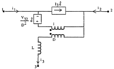
Fig. 3. The DC and AC small-signal averaged model of the converter-cell that was shown in Fig. 2.
It is shown that a DC and AC small-signal averaged model of the converter-cell which is shown in Fig. 2, can be produced as shown in Fig. 3, where D is the DC value of the duty ratio, dˆ is the small-signal perturbation of the duty ratio,
and V32 is the DC voltage between terminals 3 and 2.
The DC and AC small-signal averaged model, shown in Fig. 3, will be used to derive the corresponding output, input-to-output, input impedance, and the control-to-input current transfer functions for the Buck converter. Also, the averaged model will be used to derive the input-to-output, control-to-output, input impedance, and control-to-input current average transfer functions for the PWM Buck converter. Fig. 4 shows a typical Buck converter.
We assume a small-signal perturbation vˆ , in the DC g voltage source Vg, and that |Vg||vˆg|. After the implementation of the averaged model that was shown previously, we get the following small-signal model for the PWM Buck converter as shown in Fig. 5.
Nulling the input vˆ , we get the following control-to-g output transfer function [7]:
2 )
/ ( 1
1 ˆ
ˆ
LCs s R L V d v
g o
(1)
Nulling the input dˆ , we get the following input-to-output
[image:3.595.315.546.610.697.2]transfer function [7]:
[image:3.595.65.276.615.706.2]Fig. 5. The AC small-signal model of the Buck converter operating in the continuous conduction mode.
2 ) / ( 1 1 ˆ ˆ LCs s R L D v v g o
(2) Other transfer functions of interest for the Buck converter are the input impedance and the control-to-input current transfer functions. To get the input impedance (vˆg/iˆ), we null the input dˆ , so we get the following equation [7]:
RCs LCs s R L D R i vg 1 ) / ( 1 ˆ ˆ 2 2 1 (3) To get the control-to-input current transfer function (iˆ1/dˆ),
we null the input vˆ , so we get the transfer function [7]:g
2 2 3 3 3 3 3 g 1 ) / ( 1 ) ( ) ( 1 ˆ ˆ LCs s R L s RI D V RC LI s RI D V LI DRC V R RI D V d
i g g
g
(4)
2.1.2. New Method for Obtaining an Exact Model of the PWM Switch Within the Duty Ratio Programming Mode
In this subsection, a new approach is developed to formulate a new model for the PWM nonlinear switch [7]. The Buck converter will be used now as the basic model to extract the corresponding two-port network parameters. The main reason that the Buck is used over the other PWM converters, is the fact that the Buck converter is a second order system with a simple structure. This will be reflected upon the simplicity of the results that will be obtained.
Since the ripple voltage is comparatively much smaller than the DC voltage across the output capacitor (as the Buck converter is operating in the CCM), the capacitor will be replaced with a constant DC voltage source Vc´p. This is illustrated in Fig. 6.
[image:4.595.309.555.103.273.2]From the Buck converter shown in Fig. 6, the two-port augmented equations can be written as follows:
Fig. 6. An alternative Buck configuration.
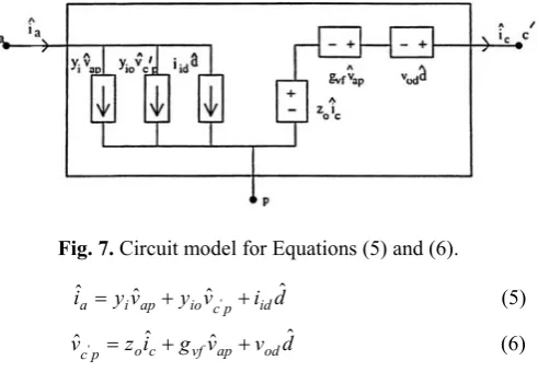
Fig. 7. Circuit model for Equations (5) and (6).
iˆa yivˆapyiovˆc'piiddˆ (5) d v v g i z
vˆc'p oˆc vfˆap odˆ (6) A circuit model for the two-port augmented equations, which are represented by Equations (5) - (6), can be constructed as shown in Fig. 7.
The aim is to develop a new model for the PWM switch, which is the nonlinear part of the PWM converter. This model can be constructed directly by replacing the values of the parameters {yi, yio, iid, zo, gvf, vod} in their simplest form [7] in Equations (5) - (6). Thus, the mathematical model will be as follows [7]:
iˆa yivˆapyiovˆc'piiddˆ d L V j I v L jD v L T DT j DT j ap x p c ap ˆ ) 1 ( ) 1 ( ˆ ˆ ) 1 ( -1 + ) 1 ( 2 1 1 2 2 1 2 s 2 1 s s 2 1 ' (7) d V v D i L j d v v g i z v ap ap c od ap vf c o p c ˆ ˆ ˆ ˆ ˆ ˆ ˆ'
[image:4.595.312.548.414.507.2] (8) By noting that the parameter zo represents an inductor, we can “pull” the zo parameter outside the circuit model, which is equivalent to the mathematical model which is represented by Equations (7) - (8), as the zo parameter is merely an inductor impedance, which is then multiplied by the corresponding path current iˆ , to form a voltage source (c zoiˆ ) in series with the c voltage sources (gvfvˆ ) and (ap vod dˆ ). The result of this process is shown in Fig. 8.
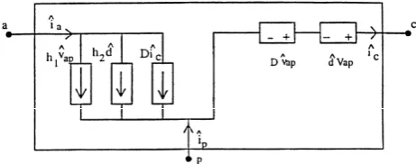
[image:4.595.45.293.637.722.2]Fig. 9. Circuit model for the PWM switch.
From Fig. 8, we can recognize that the circuit model between the terminals {a, p, c} is merely the switch between these terminals in the original Buck converter circuit. So, the equivalent switch model in terms of the perturbations {vˆ ,ap
p c
vˆ' , dˆ } is shown in Fig. 9. Now we need to obtain the
switch model in terms of the perturbations {vˆ ,ap vˆ , cp dˆ }
instead of the perturbations {vˆ ,ap vˆc'p, dˆ }. To do so, we note
from Fig. 8 that:
c cp p
c v j Li
vˆ' ˆ ˆ (9)
From Fig. 8, we note that the common node (c´) corresponds to the node (c´) in the Buck converter in Fig. 6. After multiplying both sides of Equation (9) by the parameter
yio, we get:
c cp io p c
iov y v Di
y ˆ' ˆ ˆ (10) So, we can replace the term {yiovˆcpDiˆc} instead of the term {yiovˆc'p} in the previously derived switch model shown
in Fig. 9, in order to make the new model contains the perturbations {vˆ ,ap vˆ , cp dˆ } instead of the perturbations {vˆ ,ap vˆc'p, dˆ }. The new switch model will be constructed as
shown in Fig. 10.
[image:5.595.307.538.614.705.2]In order to reduce the number of the dependent current sources that appear in the new switch model, which are four dependent current sources, we will try to reduce the number of terms in the previous mathematical switch model. One has:
Fig. 10. Alternative circuit model for the PWM switch.
ap ap
cp V d Dv
vˆ ˆ ˆ (11) and as (vˆc'p zoiˆcgvfvˆapvoddˆ), we obtain:
c ap ap
p
c V d Dv j Li
vˆ' ˆ ˆ ˆ
(12)
To develop the first reduced mathematical switch model, we note that iˆayivˆapyiovˆc'piiddˆ. Substituting Equation
(12) in Equation (5), and after the collection of the similar terms, we get the following reduced-form equation:
c io id ap io ap io i
a y y Dv y V i d jy Li
iˆ ( )ˆ ( )ˆ ˆ (13)
Substituting the values of {yi, yio, iid} in Equation (13), we get the following equation [7]:
ap v L jD T j e L T T D j e DT j e DT j DT j T j e i ˆ ) 1 ( 1 ) 1 ( ˆ 2 s 2 s s s s s s '
j T d Dic e L p Va DT j e T D j je L p jDVa x
I ˆ ˆ
) s 1 ( ) s 1 ( s ' (14)
The other equation of the model is Equation (11). So, Equations (11) and (14) represent the final reduced mathematical model of the PWM switch, replacing the model represented in Fig. 9. The final equivalent circuit model of the switch mathematical model (which is represented by Equations (11) and (14)) is as shown in Fig. 11 [7], where:
L jD T j e L T T D j e DT j e DT j DT j T j e h 2 ) s 1 ( 2 s s s s 1 ) s 1 ( s
1
' (15) ) 1 ( ) 1 ( s s s
2 j T
e L V DT j e T D j je L jDV I
h x ap ap
' (16)
The new switch model in Fig. 11 is expected to be an exact small-signal model since the mathematical equations, upon which the whole derivation process was built, are exact. Also, one notes that two of the dependent current sources are frequency dependent, which is uncommon for current or voltage dependent sources.
2.1.3. Examining the New Small-Signal Model: The Implementation of the New Small-Signal Model of the
PWM Switch on the Buck DC-DC Power Converter
In this subsection, the new small-signal model of the PWM switch, that was developed in the previous sub-section, will be examined on the PWM Buck converter. The control-to-output, input-to-output, input impedance, and control-to-input current transfer functions will be derived for the Buck converter, using the new small-signal model of the PWM switch. These transfer functions will be compared to the corresponding transfer functions for the averaged modeling approach and the exact transfer functions for the Buck converter.
By applying the PWM switch model that was developed previously for the Buck power converter, one obtains the equivalent circuit model as shown in Fig. 12.
We assume that the input DC voltage source, Vg, has small-signal perturbation, vˆ , and that g |Vg||vˆg|. To determine the system quadruple {[A], [B], [C], [E]} for the Buck model shown in Fig. 12, for the inputs dˆ and vˆ , we null the DC g voltage source Vg. Then, the following equations can be developed for the Buck model shown in Fig. 12, where iˆ is l
the inductor current, iˆ is the capacitor current, and c iˆ is the o output current that flows in the output resistor. Hence, we have the following equations:
vˆovˆc, iˆliˆciˆo c vo
R v Cˆ 1 ˆ
(17)
c l c v RC i C
vˆ 1 ˆ 1 ˆ
(18)
g
ap v
vˆ ˆ (19)
DvˆgdˆVgLiˆlvˆc0
c g g l v L d L V v L D
iˆ ˆ ˆ1 ˆ
(20) The output equation is (yvˆo vˆc). For the converter states x
and inputs u, where x = o l v i ˆ ˆ
and u = d vg ˆ ˆ
[image:6.595.48.292.390.679.2], the system quadruple {[A], [B], [C], [E]} will be [7]:
Fig. 12. Equivalent circuit model of the PWM Buck converter, which is obtained through the application of the new small-signal model of the PWM switch.
1/RC 1/C 1/L 0
A ,
0 0 /L V D/L g
B , C
0 1,
0 0
E .
To find the control-to-output transfer function, we null the input vˆ . The new system quadruple {[g A], [B], [C], [E]} will be as follows [7]:
A= 1/RC 1/C 1/L 0 (21) B= 0 /L Vg (22)
C=
0 1
(23)E=
0 (24) To find the control-to-output transfer function from the system quadruple represented by Equations (21) - (24), we apply the Laplace transformation to both sides of the state and output equations represented by system state space equations) ( ) ( )
(t Axt Bu t
x and y(t)Cx(t)Eu(t). After re-arranging the resulting terms, we get the following general input-to-output transfer function:
E B A s C u y
( Ι )1 (25) By applying Equations (21) - (24) in Equation (25), for the circuit values of {Vg = 15 V, R = 18.6 , D = 0.4, fs = 40.3 kHz, D´ = 1 – D = 0.6, L = 58 µH, C = 5.5 µF}, and to investigate the accuracy of the new PWM switch model, we compare the control-to-output frequency response plots of the PWM Buck converter, which is obtained through the application of the new PWM switch small-signal model, with both of the exact and the averaged control-to-output frequency responses, as shown in Fig. 13.
To get the input-to-output transfer function, we null the inputdˆ . The system quadruple {[A], [B], [C], [E]} will be as follows [7]: A= 1/RC 1/C 1/L 0 (26)
B =
0 D/L (27)
C =
0 1
(28)E =
0 (29) By applying Equations (26) - (29) in Equation (25), for the circuit values of {R = 18.6 , D = 0.4, fs = 40.3kHz, D´
Fig. 13. The control-to-output magnitude and phase frequency response plots of the PWM Buck converter operating in CCM: exact (solid line), averaged (dotted line), and the new model (dashed line).
From the previous frequency response plots for both of the control-to-output and the input-to-output transfer functions of the PWM Buck converter, which is operating in the CCM, we see that an excellent match occurs between the exact and the new model results, as well as between the averaged and the new model results.
These results indicate, for the time being, that the newly utilized small-signal model of the PWM switch is, in fact, an accurate model [7].
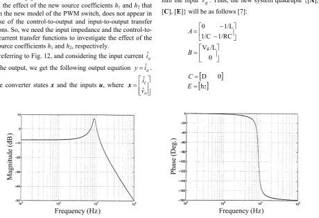
Yet, the effect of the new source coefficients h1 and h2 that
exist in the new model of the PWM switch, does not appear in the case of the control-to-output and input-to-output transfer functions. So, we need the input impedance and the control-to-input current transfer functions to investigate the effect of the new source coefficients h1 and h2, respectively.
By referring to Fig. 12, and considering the input current iˆ a to be the output, we get the following output equation yiˆa. For the converter states x and the inputs u, where
o l
v i
ˆ ˆ
x
and
d vg
ˆ ˆ
u , the system quadruple {[A], [B], [C], [E]} will
be as follows [7]:
1/RC 1/C
1/L 0
A ,
0 0
/L V
D/L g
B , C
D 0
,
h1 h2
E .
To find the control-to-input current transfer function, we null the input vˆ . Thus, the new system quadruple {[g A], [B], [C], [E]} will be as follows [7]:
1/RC 1/C
1/L 0
A (30)
0
/L Vg
B (31)
D 0
C (32)
h2
E (33)
[image:7.595.71.532.398.713.2]
Fig. 15. The control-to-input current magnitude and phase frequency response plots of the PWM Buck converter operating in CCM: exact (solid line), averaged (dotted line), and the new model (dashed line).
To find the control-to-input current transfer function from the system quadruple represented by Equations (30) - (33), we use the general input-to-output transfer function which is represented by Equation (25).
By applying Equations (30) - (33) in Equation (25), for the circuit values of {Vg = 15V, R = 18.6 , D = 0.4, fs = 40.3 kHz, D´ = 1 – D = 0.6, L = 58 µH, C = 5.5 µF}, and to investigate the accuracy of the new PWM switch model, we compare the control-to-input current frequency response plots of the PWM Buck, which is obtained through the application of the new PWM switch small-signal model, with both of the exact and the averaged control-to-input current frequency responses, as shown in Fig. 15.
To obtain the input impedance transfer function, we null the inputdˆ . Thus, the system quadruple {[A], [B], [C], [E]} will be as follows [7]:
1/RC 1/C
1/L 0
A (34)
0 D/L
B (35)
D 0
C (36)
h1
E (37) By applying Equations (34) - (37) in Equation (25), for the circuit values of {Vg = 15V, R = 18.6, D = 0.4, fs = 40.3 kHz, D´ = 1 – D = 0.6, L = 58 µH, C = 5.5 µF}, and to investigate the accuracy of the new PWM switch model, we compare the input impedance frequency response plots of the PWM Buck, which is obtained through the application of the new PWM switch small-signal model, with both of the exact and the averaged input impedance frequency responses, as shown in Fig. 16.
From the previous frequency response plots of the transfer functions of the PWM Buck converter, operating in the CCM, we see that a good match occurs between the exact and the
new model results, as well as between the averaged and the new model results, for the frequency range up to half of the switching frequency [7], although a mismatch occurs between the exact and the new model results, as well as between the averaged and the new model results, for the frequency range higher than half of the switching frequency [7].
Yet, in an overall performance evaluation, the new small signal model behaves in a much accurate response than the older averaged modeling approach.
2.2. Fuzzy Logic
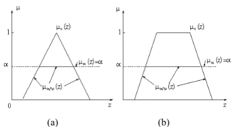
Fuzzy logic can be considered as an efficient tool for embedding structured (human) knowledge into useful algorithms that has a large number of existing applications in human sciences, natural sciences, and engineering applications [1, 6, 14, 15, 17, 19-20, 23-25, 28, 34, 35, 37, 40, 43-47, 49, 53, 54, 57- 59, 61, 63, 64, 66-67, 70-71, 76, 79, 80, 84, 86, 88-89, 92, 94-100]. It is a precise engineering tool developed to do a good job of trading off precision and significance. As in human reasoning and inference, the truth of any statement, measurement, or observation is a matter of degree. This degree is expressed through the membership functions that quantify (measure) the degree of belonging of some (crisp) input to given fuzzy subsets. Fig. 17 shows the difference between crisp set used in crisp logic and fuzzy set used in fuzzy logic.
A fundamental notion within set theory is that of belonging or membership. In the classical crisp convention, there are two possibilities that x belongs to A or it does not. This can be compared to fuzzy notion where a membership function describes the degree of belonging. Thus, crisp sets all have precise boundaries, where fuzzy sets have imprecise boundaries. The membership µ is “0” or “1” for the crisp sets
and (0 1) for the fuzzy sets. For Fig. 17(a), the set is crisp in that:
otherwise ,
0 ,
1 x1 x x4
Fig. 16. The input impedance magnitude and phase frequency response plots of the PWM Buck converter, operating in CCM: exact (solid line), averaged (dotted line), and the new model (dashed line).
[image:9.595.309.545.551.686.2](a) (b)
Fig. 17. An example of two types of sets: (a) crisp set and (b) fuzzy set.
otherwise ,
0 , 1
and ],
1 , 0 [
3 2
4 3
2 1
x x x
x x x x x x
(39)
Like crisp sets, fuzzy sets are subject to set operations such as union, intersection and complement. There are many functions that describe the union and intersection operations, where the mostly used ones in fuzzy logic are the max and min
functions as follows:
Union: C(x)AB(x)max[A(x),B(x)] (40) Intersection:
C(x)AB(x)min[A(x),B(x)] (41) As previously stated, fuzzy logic is based on representing human reasoning as a classical binary relation. The concept of relation is general; it is based on the concept of ordered pairs (a, b), where a relation from A to B (or between A and B) is any subset
of the Cartesian product A x B. We say that {aA,bB} are related by
.Fuzzy logic is usually expressed in terms of (if … and …
then) form. Fig. 18 shows an example of this (if … and …
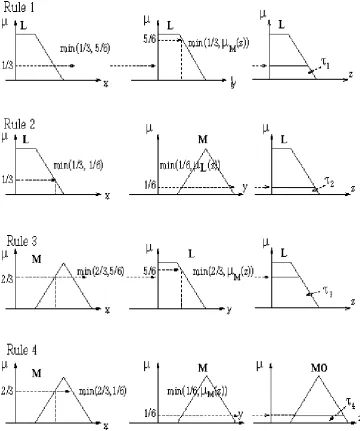
then) rule where the actual meaning of the (if … and … then) rules is (ifx is Aiandy is Bj thenz is Ck).
In fuzzy logic, the mathematical interpretation of AND is the intersection. For example, the intersection of Ai and Bj is treated using the min function as follows:
AiBj min( Ai, Bj) (42)
The membership value α is called the power of the rule or the firing power. This part is then intersected with Cij to simulate the “then” part of the (if…and…then) rule. This intersection is expressed as a clipped fuzzy rule as shown in Fig. 19.
A crisp input can cause the firing of several rules. This is interpreted as the aggregation or union of these rules, where the final part of the aggregation of the rules is usually interpreted as the max operation. An example of rule aggregation is shown in Fig. 20, and Fig. 21 shows an example of firing rules within fuzzy logic.
The final part which is usually utilized within fuzzy implementation is defuzzification. The defuzzification process has several techniques including the center of area method where we divide the area into equally spaced rectangles and for each we find the membership function. This is shown for the rule aggregation in Fig. 20.
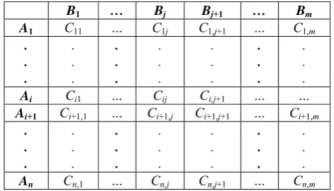
B1 … Bj Bj+1 … Bm
A1 C11 … C1j C1,j+1 … C1,m
. . .
. . .
. . .
. . .
. . .
. . .
. . .
Ai Ci1 … Cij Ci,j+1 … …
Ai+1 Ci+1,1 … Ci+1,j Ci+1,j+1 … Ci+1,m
. . .
. . .
. . .
. . .
. . .
. . .
(a) (b)
Fig. 19. Clipped triangular and trapezoidal membership
functions.
zk 10 20 30 40 50 60 70
µagg 2/3 2/3 2/3 1/3 1/6 1/6 1/6
For the above example, when implementing the defuzzification, using the center of area method, one obtains the defuzzified value as follows:
41 . 29 6 1 6 1 6 1 3 1 3 2 3 2 3 2 6 1 70 6 1 60 6 1 50 3 1 40 3 2 30 3 2 20 3 2 10 ) ( ) ( 1 1 1 1
q k k agg q k k agg k c z z z z 2.3. Genetic Algorithms
This subsection provides a basic background for the evolutionary-based algorithms. In general, evolutionary computing (EC) is one type of “black box” global optimization methods that has been successfully implemented to solve for many difficult nonlinear problems. An EC implements the idea which was proposed by Darwin as an explanation of the biological world surrounding us which is the "Evolution by Natural Selection". By evolution, we mean the change of the genes that produce a structure. The result of this evolution is the survival of the fittest and the elimination of the unfit. Darwin's theory of evolutionary selection states that variation within species occurs randomly and that the survival or extinction of each organism is determined by that organism's ability to adapt to its environment.
This simple, but powerful, EC idea has been implemented in algorithms such as genetic algorithms (GA) and genetic programming (GP), and found wide spectrum of applications in several natural and applied fields [18, 21, 22, 24, 26, 27, 29, 33, 36, 41, 42, 44, 48, 50-52, 55, 56, 59-62, 68-69, 72-75, 78, 81-83, 85, 87, 91]. The difference between GA and GP is the representation of the problem and consequently the set of genetic operators used to obtain the solution; GA uses string
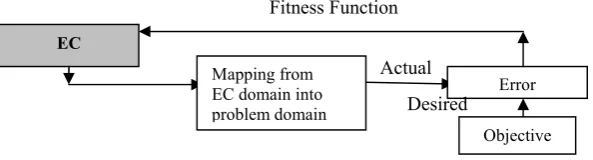
representation and the consequent genetic operators, while GP uses tree representation and the consequent genetic operators. Fig. 22 represents the general optimization using the EC method, where iterations on this flow diagram are made until the actual output matches exactly the desired output (i.e., without error) or the actual output mismatches the desired output within an acceptable range of error.
In general, GA is based on the simulation of life, where the first step is usually to represent the problem variables as chromosomes also called genomes. The basic steps and common operations within GAs are as follows (cf. Fig. 23): (a) Initialization: within this step, the chromosomes are generated randomly to cover the search space and in some special cases the population is seeded with special solution or optimal solutions.
(b) Selection: there are several types used for selection such as: (1) fitness proportionate selection or roulette-wheel selection (a single random number is used), (2) stochastic universal sampling (multiple random numbers are generated for selection), (3) tournament selection (best individuals are always selected), (4) truncation selection (a portion of the population is selected), and (5) elitism or elitist selection (where the best individual(s) are always selected).
(c) Crossover: this operation involves the combination of genes from two parents to produce offsprings. There are several variants of crossover: (1)single point crossover where a fixed position is selected in both parents and then the contents beyond that crossover point are swapped, (2) multiple crossover points, (3) cut and slice crossover (change in length between the parents and the children), and (4) uniform crossover where a random number is generated and, if it is greater than a threshold value, then swapping is performed. (d) Mutation: this process involves the reproduction of an erroneous copy of the individual, in which a random number is generated where if it is greater than a threshold value then the zero binary value is changed to one. This part is added to increase the diversity.
(e) Copying: this process involves the reproduction of an exact copy of the individual.
[image:10.595.363.510.586.707.2](f) Termination: where a certain number of generations is reached, or an acceptable solution is reached, or no change in the optimal solution is reached.
Fig. 22. Block diagram showing the mechanism of problem solving utilizing evolutionary computing.
Fig. 23. A flow graph of a generally-used genetic algorithm. EC
Mapping from EC domain into problem domain
Error Actual
Objective Fitness Function
Desired
Run:=0
Gen.:=0
Create Initial Population (Random,Seeding,or Hybrid)
for Run (Strings:Binary/MV and Fixed/Variable length)
Termination Criterion is Satisfied for Run
No
Yes Designate
Result for Run Run:=Run+
1 Run=N?
No
END
Yes
Evaluate Fitness of each Individual
in Population.
i:=0
i=M?
Yes
No
Gen.:=Gen.+1
Select Genetic Operation
Copy into new population Perform Reproduction
on copy of Indiv.
Prf1(Fitness)
Select one individual based on fitness (with reselection allowed)
Pcf2(Fitness)
Select Two Indiv. (Parents) based on fitness (with reselection allowed)
i:=i+1
Select Crossover point (Fixed/Random and Single/Multiple)and perform crossover (Sexual Recombination) on copy of Indiv.
Insert Two Offspring into the new population
Pmf3(Fitness)
Select one individual based on fitness (with reselection allowed)
Perform Mutation on copy of Indiv. (Fixed/Random and Single/Multiple Mut. Point)
Insert Mutant into the new population
i:=i+1
Loop 3 Loop 2
[image:12.595.127.455.259.685.2]
Fig. 24. A canonical flow graph for evolutionary methods. Fig. 23 demonstrates a general flow diagram of an EC, where Run is the current run number, N is the maximum number of runs, Gen. is the current generation number, M is the population size, i is the current individual in the population, Pr is the probability of reproduction, Pc is the probability of crossover, Pm is the probability of mutation, and (Pr + Pc + Pm= 1.0). In Fig. 23, the result of looping over Gen. is the best-of-run individual, the result of looping over Run is the best-of-all individual, and the result of looping over i is the best-of-generation individual. Iterations in Fig. 23 continue until an optimal solution is obtained. Since the EC algorithms are try-and-check (i.e., try-and-error) probabilistic search algorithms (i.e., depends on the reduction of error in the search process to produce a solution), the EC program may have to perform so many iterations (as in Fig. 23) to produce the desired solution to a problem. Thus, and although EC methods produce in many occasions new solutions that humans never made before, it is in general highly advisable to consider EC as one final option for problem solving (i.e., when other methods fail to solve the problem), since EC acts like a “black box” that produces solutions without showing methodology (i.e., EC does not provide a detailed step-by-step algorithm (analytical or procedural) to solve a problem and it only shows the final solution).
The evolutionary algorithm from Fig. 23 has many variants. Yet, a canonical form for all of these variants exist. Fig. 24 illustrates one possible canonical diagram for evolutionary computing, where selecting survivors means (1) selection of parents and (2) generation of offspring.
The canonical diagram for EC (shown in Fig. 24) characterizes the canonical implementation of various types of EC such as GA, and as stated previously, the only difference between GA and other EC (such as the GP) will be in (1) the internal representation of chromosomes operated upon and (2)
the types of internal operations used accordingly. Fig. 25 shows an example of some important GA operations.
3. GENETIC–BASED TUNING FOR THE BUCK–
BASED FUZZY CONTROL
This section presents the basic used Simulink and MATLAB setups, and the GA-based tuning of the fuzzy controller, that will be used in Section 4 to obtain the fuzzy-PID control results.
3.1. Simulink and MATLAB Setups
In MATLAB, solvers are divided into two main types of (a) fixed-step solvers and (b) variable-step solvers. Both types of solvers compute the next simulation time as the sum of the current simulation time and a quantity known as the step size. With a fixed-step solver, the step size remains constant throughout the simulation. On the contrast, with a variable-step solver, the variable-step size can vary from variable-step to variable-step, depending on the model's dynamics. In particular, a variable-step solver reduces the step size when the model's states are changing rapidly in order to maintain accuracy and increases the step size when the system's states are changing slowly in order to avoid taking unnecessary steps.
The type of control within the Simulink solver configuration allows selecting either of these two types of solvers. Fixed-step solvers have lower chances of missing an event in the model as compared to a variable-step solver that may cause the simulation to miss error conditions that can occur on a real-time computer system. Thus, for this work, fixed-step solvers are used for a step size of 0.001s to ensure capturing all of the dynamics occurring in the Buck system. If the step size is chosen less than this value, it will be highly time consuming for the GA code to run as the model will take large amount of time to run. Other step-size values such as 0.01s were tested but the model results were not as accurate as that of 0.001s.
Another configuration for the MATLAB solvers is (a) continuous time and (b) discrete time, where continuous time solvers can handle both of the discrete and continuous blocks which is the case for the analyzed system.
Thus, we have chosen the continuous solvers. Within the prospect of continuous systems, we can use (a) implicit solvers or (b) explicit solvers by using implicit or explicit functions. The implicit solvers are more time consuming than explicit solvers, and thus explicit solvers were used with the Runge-Kutta (RK4) model because of the optimization part.
3.2. Genetic–Based Tuning for the Centers of Fuzzy Membership Functions
For this case, the centers in Fig. 26 for the inputs and outputs can be set by the GA algorithm and not the gains {ke,
kde, Alpha, Beta}. The Simulink is then executed with the
generated fuzzy logic variable. The sum-of-square error (SSE) is calculated as the fitness value.
Evaluate Fitness
Select Survivors
Randomly Vary Individuals
Fig. 25. An illustrative example of important GA operations.
[image:14.595.101.506.502.671.2]Fig. 27. The utilized Simulink block diagram for the GA-based tuning of the fuzzy variables within the Buck system.
Then the GA, which was explained earlier, regenerates a new population using the selection, crossover and mutation genetic operators. However, this can lead to lengthy GA runs and thus the convergence time for the GA could be very high. Therefore, this setup was not used in this research.
3.3. Fuzzy PID Case: Genetic–Based Tuning for the Fuzzy Variables
As an alternative to the method shown in sub-section 3.2, Fig. 27 shows the Simulink block diagram that is used in this work for the GA tuning of the fuzzy-PID variables, where GA changes the chromosomes for tuning the fuzzy variables (cf. Fig. 29). The fuzzy-PID method shown in Fig. 27 is a standard commonly used PID control form which is utilized in several other applications [15, 24, 44].
4. GENETIC–BASED TUNING FOR THE FUZZY
VARIABLES OF THE BUCK CONVERTER
This section presents the simulation results for the GA tuning of the fuzzy variables for both of the input–to–output and control–to–output Buck transfer functions.
4.1. Genetic–Based Tuning for the Fuzzy Variables for the Input-to-Output Buck Transfer Function
[image:15.595.305.545.536.672.2]In Fig. 27, the error is calculated first using the summing function as the difference between the input and the output. Followed to that, the proportional part and the derivative part are calculated and multiplied by the counterpart gain {ke, kde}.
Fig. 28. Fuzzy sets for the error, derivative and the output.
Then, this is used as an input to a multiplexer, and then these two inputs (i.e., proportional and derivative) are used as an input to the fuzzy logic part. These are then fuzzified using the fuzzy sets and membership functions shown in Fig. 28.
The fuzzified variables are then processed using the Mamdani-type fuzzy system using the rules in Table (1). The centroid type defuzzification system is then estimated. The output is then multiplied by the corresponding gains {Alpha, Beta} and then integration is used.
Fig. 29 shows the block diagram of the interaction between the genetic algorithm part and the fuzzy-PID controller part that is used in this work, and Fig. 30 illustrates a sample run for the utilized fuzzy control. The GA is based on representing the different parameters {ke, kde, Alpha, Beta} as a
[image:15.595.44.292.599.699.2]chromosome. The fuzzy-PID controller runs the model with the selected values for these parameters and passes the output to an M-file which estimates the sum of the square error (SSE). This in turn is treated as the fitness function. The GA then performs the genetic operations of selection, crossover and mutation on the chromosomes and produces a new population which in turn uses the fuzzy-PID controller model to estimate the fitness. This cycle continues until a suitable minimum value is reached for termination.
Table 1. Rules for the utilized Mamdani-type fuzzy system.
Fig. 31 presents the simulation results for the input-to-output Buck transfer function using the state space matrices
{A =
1/RC 1/C
1/L 0
, B =
0 D/L
, C =
0 1
, E =
0 } and using the Buck system values of {D = 0.4, R = 18.6, L = 5.8 H, C = 0.55 mF} with noisy input for a step function and square wave functions, where the noise in the first square wave is 0.1:1 of the signal, the noise in the second square wave is 1:1 of the signal, and the noise in the third square wave is 10:1 of the signal.
[image:16.595.61.540.431.588.2]0 5 10 -0.2
0 0.2 0.4 0.6 0.8 1 1.2
Time
R
e
s
pons
e
0 5 10
-2 0 2
Time
R
e
s
pons
e
0 5 10
-2 0 2
Time
R
e
sp
o
n
se
0 5 10
-2 0 2
Time
R
e
sp
o
n
se
0 5 10
-2 0 2
Time
R
e
s
pons
e
0 5 10
-2 0 2
Time
R
e
sp
o
n
se
0 5 10
-2 0 2
Time
R
e
sp
o
n
se
[image:17.595.147.459.106.372.2](a) (b) (c)
Fig. 31. Simulation results for the Buck input-to-output using system values {D = 0.4, R = 18.6, L = 5.8 H, C = 0.55mF}.
0 5 10
-0.2 0 0.2 0.4 0.6 0.8 1 1.2
Time
R
e
sp
o
n
se
0 5 10
-2 -1 0 1 2
Time
R
e
sp
o
n
se
0 5 10
-2 -1 0 1 2
Time
R
e
sp
o
n
se
0 5 10
-2 -1 0 1 2
Time
R
e
sp
o
n
se
0 5 10
-2 -1 0 1 2
Time
R
e
sp
o
n
se
0 5 10
-2 -1 0 1 2
Time
R
e
sp
o
n
se
0 5 10
-2 -1 0 1 2
Time
R
e
sp
o
n
se
(a) (b) (c)
[image:17.595.144.459.411.680.2]
0 5 10
-0.2 0 0.2 0.4 0.6 0.8 1 1.2
Time
R
e
s
pons
e
0 5 10
-2 0 2
Time
R
e
s
pons
e
0 5 10
-2 0 2
Time
R
e
s
pons
e
0 5 10
-2 0 2
Time
R
e
s
pons
e
0 5 10
-2 0 2
Time
R
e
s
pons
e
0 5 10
-2 0 2
Time
R
e
s
pons
e
0 5 10
-2 0 2
Time
R
e
s
pons
e
[image:18.595.142.448.85.344.2](a) (b) (c)
Fig. 33. Simulation results for the Buck control-to-output using system values {Vg = 15 V, C = 1 mF, R = 1 k, L = 5.8 H}. To ensure that the system is tested well, different type of
inputs were used including (a) step input in Fig. 31(a), (b) 0.2 Hz pulse input with noise levels {0.1:1, 1:1, 10:1} in Fig. 31(b), and (c) 0.4 Hz pulse input with noise levels {0.1:1, 1:1, 10:1} in Fig. 31(c). The different noise levels are used to test the ability of this system to reject the existing noise.
Fig. 31 shows that the system has good robustness against noise and possesses good accuracy for the steady-state reponse. However, the settling time is somewhat high, where these values are obtained as a result of the optimization process and shows the best obtained performace that the system can perform under the aforementioned condititions.
To further investigate the system, different Buck system values of {D = 0.4, R = 18.6 , L = 580 mH, C = 55µF} were used for (a) step input in Fig. 32(a), (b) 0.2 Hz pulse input with noise levels {0.1:1, 1:1, 10:1} in Fig. 32(b), and (c) 0.4 Hz pulse input with noise levels {0.1:1, 1:1, 10:1} in Fig. 32(c). The different noise levels are used to test the ability of this system to reject the occurring disturbances. Fig. 32 shows the performance of the Buck converter system which is represented by the state- space matrices {A=
1/RC 1/C
1/L 0
, B
=
0 D/L
, C =
0 1
, E =
0 } using the previously mentioned values with noisy inputs for a step function and square wave functions, where the noise in the first square wave is 0.1:1 of the signal, the noise in the second square wave is 1:1 of the signal, and the noise in the third square wave is 10:1 of the signal. The system shows a low steady-state error, but bad noise rejection especially for high noise level of 10:1 when compared to the signal. The response time is comparable to that in Fig. 31 for the previous Buck system. The system gets worse for high-frequency values as the final steady-state value might not be reached for the used step time.
4.2. Genetic–Based Tuning for the Fuzzy Variables for the Control-to-Output Buck Transfer Function
The Buck dynamic system is then tested for the important control-to-output transfer function as shown in Fig. 33, where Fig. 33 presents the simulation results for the control-to-output
Buck transfer function using the state space matrices
{A =
1/RC 1/C
1/L 0
, B =
0 Vg
, C =
0 1
, E =
0 } with values {Vg = 15 V, C = 1 mF, R = 1 k, L = 5.8 H}. The Buck system is simulated for different types of inputs including (a) step input in Fig. 33(a), (b) 0.2 Hz pulse input with noise levels {0.1:1, 1:1, 10:1} in Fig. 33(b), and (c) 0.4 Hz pulse input with noise levels {0.1:1, 1:1, 10:1} in Fig. 33(c). The different noise levels are used to test the ability of this system to reject the corresponding noise.0 5 10 -0.2
0 0.2 0.4 0.6 0.8 1 1.2
Time
R
e
s
p
ons
e
0 5 10
-2 -1 0 1 2
Time
R
e
s
pon
s
e
0 5 10
-2 -1 0 1 2
Time
R
e
s
p
ons
e
0 5 10
-2 -1 0 1 2
Time
R
e
s
pon
s
e
0 5 10
-2 -1 0 1 2
Time
R
e
s
pon
s
e
0 5 10
-2 -1 0 1 2
Time
R
e
s
p
ons
e
0 5 10
-2 -1 0 1 2
Time
R
e
s
pon
s
e
[image:19.595.149.452.84.355.2](a) (b) (c)
Fig. 34. Simulation results for the Buck control-to-output using system values {Vg = 20 V, C = 2 mF, R = 3 k, L = 11 H}. To further investigate the Buck system performance,
different Buck values of {Vg = 20 V, C = 2 mF, R = 3 k, L = 11 H} were used. The Buck system is simulated for different types of inputs including: (a) step input in Fig. 34(a), (b) 0.2 Hz pulse input with noise levels {0.1:1, 1:1, 10:1} in Fig. 34(b), and (c) 0.4 Hz pulse input with noise levels {0.1:1, 1:1, 10:1} in Fig. 34(c), where the different noise levels are used to test the ability of this system to reject noise. Similar to Fig. 33, the results in Fig. 34 show an acceptable steady-state Buck performance despite small overshoots that have usually a comparatively negligible effect on the overall performance.
5. CONCLUSION
Hierarchical intelligent regulation for the electronic Buck power converter using a newly developed small-signal model of the pulse width modulation switching is introduced in this article. The hierarchical intelligent control uses the GA-based tuning of the fuzzy-PID controller to counteract the existence and effect of high-amplitude noise. The simulation results show that the presented control method, which is utilized using the new PWM small-signal model, succeeds in minimizing the effect of noise even when noise is of several levels higher than the Buck-generated output signal.
REFERENCES
[1] S. C. Abou, M. Kulkarni, and M. Stachowicz, "Actuated Hydraulic System Fault Detection: A Fuzzy Logic Approach,"Engineering Letters, 18:1, February 2010.
[2] K.K. Ahn and N.B. Kha, "Modeling and Control of Shape Memory Alloy Actuators Using Preisach Model, Genetic Algorithm and Fuzzy Logic,"
Mechatronics, Vol. 18, pp. 141–152, 2008.
[3] E. Akın, M. Kaya and M. Karakose, "A Robust Integrator Algorithm With Genetic Based Fuzzy Controller Feedback for Direct Vector Control,"
Computers and Electrical Engineering, Vol. 29, pp. 379–394, 2003.
[4] M.S. Alam and M.O. Tokhi, "Hybrid Fuzzy Logic Control With Genetic Optimization for a Single-Link Flexible Manipulator," Engineering
Applications of Artificial Intelligence, Vol. 21, pp. 858–873, 2008.
[5] D. Alejo, P. Maussion and J. Faucher, "Multiple Model Control of a Buck Dc/Dc Converter," Mathematics and Computers in Simulation, Vol. 63, pp. 249–260, 2003.
[6] H. Aljoumaa, and D. Soffker, "Multi-Class Classification Approach based on Fuzzy-Filtering for Condition Monitoring," IAENG International
Journal of Computer Science, 38:1, pp. 66-73, February 2011.
[7] A.N. Al-Rabadi, An Approach to Exact Modeling of the PWM Switch, M.Sc. Thesis, Electrical and Computer Engineering Department, Portland State University, 1998.
[8] A.N. Al-Rabadi, "Intelligent Control of Singularly-Perturbed Reduced Order Eigenvalue-Preserved Quantum Computing Systems via Artificial Neural Identification and Linear Matrix Inequality Transformation," IAENG International Journal of Computer Science
(IJCS), Vol. 37, No. 3, pp. 210 – 223, 2010.
[9] A.N. Al-Rabadi, "Artificial Neural Identification and LMI Transformation for Model Reduction-Based Control of the Buck Switch-Mode Regulator," American Institute of Physics (AIP), In: IAENG Transactions on Engineering Technologies, Special Edition of the International MultiConference of Engineers and Computer Scientists 2009, AIP Conference Proceedings 1174, Editors: Sio-Iong Ao, Alan Hoi-Shou Chan, Hideki Katagiri and Li Xu, Vol. 3, pp. 202 – 216, New York, U.S.A., 2009.
[10] A.N. Al-Rabadi, "Intelligent Control of Reduced-Order Closed Quantum Computation Systems Using Neural Estimation and LMI Transformation," Springer-Verlag, In: Intelligent Control and Computer Engineering, Special Edition of the International MultiConference of Engineers and Computer Scientists 2010, Editors: Xu Huang, Oscar Castillo, and Sio-Iong Ao, 2010.
[11] A.N. Al-Rabadi and O. M.K. Alsmadi, "Supervised Neural Computing and LMI Optimization for Order Model Reduction-Based Control of the Buck Switching-Mode Power Supply," Int. Journal of Systems
Science (IJSS), Taylor & Francis, U.S.A., Vol. 42, Issue 1, pp. 91-106,