Experimental Analysis of the Effects of Social
Relations on Mobile Application Recommendation
Tomonobu Ozaki and Minoru Etoh
Abstract—In this paper, we empirically analyze the effects of
social relations on the recommendation of mobile applications in a community of students at a university. We identify three social relations by questionnaires and two relations by students properties, and examine their effects from a wide variety of perspectives in the framework of top-N recommendation by user and item based collaborative filtering with two re-ranking mechanisms. In the analysis, we assess the difference of the effects by the origin and strength of social relations as well as by the methods of collaborative filtering and re-ranking mecha-nisms. As a result of the analysis, we confirm that appropriate social relations can significantly improve the performance of recommendation, in terms of increasing diversity and novelty with keeping high accuracy, especially for the late adopters.
Index Terms—recommendation, social relation, mobile
appli-cation
I. INTRODUCTION
R
ECOMMENDER systems attract a lot of attention as an important information technology to overcome the rapid increase of available information. Accurate and precise recommendations are absolutely necessary for the success of recommender systems.With the growth of social networks, social relations be-come to be regarded as promising information sources for improving the accuracy of recommendations [1]–[5]. For instance, the effects of social relations are deeply examined in the domain of movie recommendation [1], while the effects of different kinds of social relations are extensively compared [2], [3]. Furthermore, recommendation methods using social networks based on the collaborative filtering and the matrix factorization are developed in [4] and [5], respectively.
The results of above mentioned researches suggest that the social relations can contribute to recommender systems in terms of improving the accuracy. However, accuracy is not the only measure for the quality of recommender systems. In addition to the accurate recommendations, providing a wide range of valuable and serendipitous information is crit-ically important [6]. Researches on this topic are conducted recently. A method for diversifying recommendation lists is developed [7], while metrics for evaluating the serendipity are proposed [8]–[10]. However, the effects of social relations on recommendations are not extensively analyzed from the other perspectives than accuracy.
In this paper, we prepare five social relations having differ-ent origins and differdiffer-ent degree of strength, and empirically analyze their effects and significance on the improvement of recommendation of mobile applications from a wide variety
T. Ozaki is with Cybermedia Center, Osaka University, Japan. e-mail: [email protected].
M. Etoh is with NTT DOCOMO R&D Center, Japan. e-mail: [email protected].
Training Data
Test Data
Evaluation
Precision / Diversity / Novelty / Serendipity Recommendation Lists
( Top-N Recommendation )
Collaborative Filtering - User-based CF - Item-based CF
Re-evaluation ( Re-ranking ) Social Relations
Training Data
Test Data
Evaluation
Precision / Diversity / Novelty / Serendipity Recommendation Lists
( Top-N Recommendation )
Collaborative Filtering - User-based CF - Item-based CF
[image:1.595.304.541.161.269.2]Re-evaluation ( Re-ranking ) Social Relations
Fig. 1. Overall flow of Recommendation using Social Relations
of perspectives including accuracy, diversity, novelty and serendipity. We employ a framework of the top-N recom-mendation based on the collaborative filtering [11] with a re-ranking mechanism. In the framework, social relations are applied (1)to estimate the recommendation strength by collaborative filtering and (2)to prepare the recommendation lists by re-evaluation (re-ranking). The overall flow is shown in Fig. 1.
In the analysis, both of user based collaborative filtering methods [12]–[14] and item based ones [15]–[17] are em-ployed to compare the difference of the effects by recom-mendation methods. We also compare the differences of the effects by positions where social relations are applied, i.e. applications of social relations to (1)collaborative filtering only, (2)re-ranking only and (3)both of collaborative filtering and re-ranking.
The rest of this paper is organized as follows. In section II, we introduce the basic notations, and propose recommen-dation methods using social relations. Re-evaluation methods are also proposed. In section III, after describing the dataset and evaluation criteria, experimental results are reported. Finally, we conclude the paper and describe future work in section IV.
II. RECOMMENDATION WITHSOCIALRELATIONS
Notations used throughout the paper are summarized in Table I. Let U ={u1,· · ·, u|U|} and I = {i1,· · ·, i|I|} be
sets of users and items, respectively. Given a user x ∈ U, a set I+
x (⊆ I) denotes a set of items rated by x, while
another setIx− =I\I+
x denotes a set of items not rated by
x. A positive real number rx,i (x∈U, i∈Ix+) denotes the
rating value ofxon an item i. Given a userx∈U and an indicator functionR:U×U→ {0,1}which takes 1 if there exists a social relation R between two users, we denote a set of users having, and not having, the relationRwithxas Ux+={y ∈U : R(x, y) = 1} andUx− =U\(Ux+∪ {x}),
TABLE I NOTATIONS
Notation Description
x, y users
i, j items
U Set of all users
Ux+ Set of users having a social relation withx
Ux− Set of users not having a social relation withx
I Set of all items
Ix+ Set of items rated byx
Ix− Set of items not rated byx
rx,i Rating value ofxoni
ˆ
rx,i Recommendation strength ofiforx
sx,y Similarity betweenxandy
si,jx Similarity betweeniandjofx
α(≥0) Weight of users having social relations
β(≥0) Weight for users not having social relations
In this paper, we consider the top-N recommendation. Therefore, given a user x∈ U, the first step for obtaining the ranking list of recommendation for xis to estimate the recommendation strength rˆx,i on every item i∈Ix−. In the
following subsections, we introduce methods for estimating the recommendation strength based on the user- and item-based collaborative filtering methods by taking into account the social relations, respectively.
A. User-based Collaborative Filtering
User-based collaborative filtering methods [12]–[14] uti-lize the past ratings of similar users to estimate the recom-mendation strength. In this paper, we employ a user-based collaborative filtering based on theK-nearest neighbors.
Given two users x and y (x, y ∈ U), we propose a similarity between x and y with consideration of social relations as follows:
sx,y=
{
α·cos(x, y) (y∈U+
x)
β·cos(x, y) (y∈Ux−) (1)
whereα≥0 andβ≥0 are parameters and
cos(x, y) = ∑
i∈I+
x∩Iy+rx,iry,i √∑
i∈Ix+r
2
x,i
√∑
i∈Iy+r
2
y,i
(2)
denotes the cosine similarity based on the past ratings. The strength of social relations in calculating sx,y can be
controlled by two parameters α and β. For example, a parameter settingα= 1andβ= 0utilizes the users having social relations only, while α = β ignores the effects of social relations.
The recommendation strengthrˆx,ifor a userx∈U on an
itemi∈Ix− is derived as the weighted sum of ratings on i by the top-K similar users. Let
Ux,K ={y∈U6=x : K >|{z∈U6=x:sx,y < sx,z}|}
be a set of top-K similar users ofxwhereU6=x=U\ {x}.
Then, rˆx,iis formally defined as
ˆ
rx,i=
∑
i∈Iy+,y∈Ux,K
sx,yry,i. (3)
If we setK=|U| −1 for the K-nearest neighbors, then the user-based collaborative filtering can be formalized as a variant of the composite social network approach [18] based on the linear threshold model [19]. In the model, the probabilityP r(x, i)that a user xrates an itemi is defined as
P r(x, i) = 1−exp(−p(x, i))
where
p(x, i) = α ∑
y∈U+
x,i∈I+y
cos(x, y)ry,i+β
∑
y∈Ux−,i∈I+y
cos(x, y)ry,i
= ∑
i∈I+y,y∈Ux,|U−1| sx,yry,i
= rˆx,i.
The parameters can be estimated from the past rating behaviors by maximizing the following likelihood function under the constraints ofα≥0andβ ≥0:
∏
x∈U
∏
i∈I+x
P r(x, i)× ∏
i∈Ix−
(1−P r(x, i))
where the first and second terms correspond to the prob-abilities that each user does and does not rate the item, respectively.
B. Item-based Collaborative Filtering
Item-based collaborative filtering methods [15]–[17] uti-lize a similarity among items in general. In this subsection, we propose a personalized similarity among items with the consideration of social relations, and use it for estimating the recommendation strength.
For a set of usersU0 ⊆U, we define the cosine similarity between two itemsiandj(i, j∈I) by using the past ratings as follows:
s(i, j, U0) =
∑
x∈U0,i∈Ix+,j∈I+x rx,irx,j √∑
x∈U0,i∈Ix+r
2
x,i
√∑
x∈U0,j∈I+x r
2
x,j
. (4)
We propose a personalized similarity
si,jx = 1
α+β
(
α·s(i, j, Ux+) +β·s(i, j, Ux−)) (5)
for a userx between two items i andj. It is the weighted average over cosine similarities for U+
x and Ux− with two
parametersα≥0 andβ≥0. As the same as the similarity among users, we can control the strength of social relations in calculatingsi,jx .
The recommendation strength is derived based on the rated items. We define the recommendation strengthrˆx,iof an item
i∈Ix− for a userxas the summation of similarites between
iand a rated item j∈I+
x:
ˆ
rx,i=
∑
j∈Ix
C. Re-evaluation of Recommendation Strength by Social Relations
Besides accurate recommendations, the ability of provid-ing a wide variety of new information is one of important factors for recommendation methods [6]–[10]. According to the suggestion in [6], we propose methods for re-evaluating the recommendation strength by using social relations.
For a user x∈U and an itemi∈Ix−, the average value
of recommendation strength of i over users having social relations with xis defined as
rx,i= 1 |U(x,i)|
∑
y∈U(x,i) ˆ
ry,i
whereU(x,i)={y∈Ux+∪ {x}:i∈Iy−}.
In order to obtain high degree of diversity and novelty, the updated recommendation strength is obtained by amplifying the original recommendation strength based on the difference from the average:
ˆ
rx,i·
max(ˆrx,i, rx,i) min(ˆrx,i, rx,i)
. (7)
The method emphasizes the items having largely different recommendation strength from the average.
We prepare another re-evaluation method having the op-posite effects to obtain accurate recommendations:
ˆ
rx,i·
min(ˆrx,i, rx,i) max(ˆrx,i, rx,i)
. (8)
This method reduces the recommendation strength largely if it differs greatly from the average. As a result, the recommendation strength of ordinary items in the community increases relatively.
III. EXPERIMENTS
A. Dataset
To assess the effects of social relations on recommendation tasks, we implement all methods in Java and conduct exper-iments. We use a log data of mobile application executions collected from February to July 2011 with 157 students in Osaka University. The dataset is divided into two disjoint sets according to the timestamps. The dataset for the first three months is used to make the recommendation. After removing the log of mobile applications used by less than three students, a training data containing 377 applications with 8,576 ratings is obtained. We use the value ofln(1 + # of days whenxusesiduring the first three months) asrx,i. On
the other hand, we prepare two test data from the dataset of last three months. As the top 10% of late adopters, we select 15 active students who install at least 10 applications in the training data during the last three months. We denote the set of active students as U10. Similarly, the second test set U5 consists of 58 students who install at least 5 applications. For the training and test data, a relation U⊃U5⊃U10 holds.
We identify the following three social relations by ques-tionnaires:
1) RT: friendly enough to talk with each other,
2) RM: friendly enough to send and receive emails, and
3) RC: friendly enough to make telephone calls.
TABLE II
AVERAGE NUMBER OF USERS HAVING SOCIAL RELATIONS
RT RM RC R2 R3
U(157 students) 17.4 9.6 6.1 52.8 22.6
U5(58 students) 16.1 9.5 6.1 52.4 24.7
U10(15 students) 13.5 8.5 5.1 57.3 25.9
In addition, based on three user properties (1)gender (male or female), (2)major (art or science), and (3)location of campus (one of three places), we prepare two quasi-relations roughly capturing the homophily [20]:
1) R2: at least two properties are the same, and 2) R3: all properties are the same.
We believe that the inequalities RT < RM < RC and
R2< R3hold on the strength of social relations. The average numbers of users having social relations are summarized in Table II.
B. Evaluation Criteria
Given a set of test usersUt⊆U, the macro average
V∗(Ut) = 1 |Ut|
∑
x∈Ut
v∗(x, N)
of a measure v∗(x, N)defined below over Ut is employed as an evaluation criterion. Four evaluation measures are prepared. In the following definitions, we denote the top-N recommendation items for a userx∈U as
P(x, N) ={i∈Ix− : N >|{j∈Ix− : ˆrx,i<rˆx,j}|},
while the answer set forxis denoted as A(x) (⊆Ix−).
1) vp(x, N): The first measure is weighted precision@N,
formally defined as
vp(x, N) =
∑
i∈A(x)∩P(x,N)r0x,i
∑
i∈P(x,N)r0x,i
(9)
where
r0x,i= {
rx,i (i∈A(x))
∑
j∈A(x)rx,j/|A(x)| (i6∈A(x))
.
We use the rating value, i.e. ln(1 + # of days when x uses i during the last three months), as the weight. The average value is used for the items having no rating.
2) vd(x, N): As the second measure, we employ the
diversity, i.e. the average of cosine distance among items inP(x, N):
vd(x, N) =
∑
i∈P(x,N)
∑
j∈P(x,N),i6=j(1−s(i, j, U)) |P(x, N)|(|P(x, N)| −1) .
(10)
3) vn(x, N): The third measure is the novelty which is
defined as the average of minimum distance between rated items and predicted ones:
vn(x, N) = 1 |P(x, N)|
∑
i∈P(x,N)
min j∈I+
x
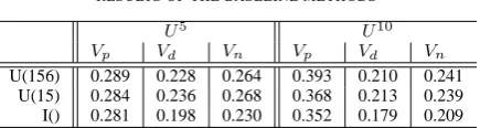
TABLE III
RESULTS OF THE BASELINE METHODS
U5 U10
Vp Vd Vn Vp Vd Vn
U(156) 0.289 0.228 0.264 0.393 0.210 0.241 U(15) 0.284 0.236 0.268 0.368 0.213 0.239 I() 0.281 0.198 0.230 0.352 0.179 0.209
4) vs(x, N): The last measure is the serendipity. It is
the ratio of correctly recommended items which are not recommended by a baseline method:
vs(x, N) = |
P(x, N)∩A(x)\P0(x, N)|
|P(x, N)| (12)
whereP0(x, N)denotes the top-N recommendation by the baseline method, i.e. the recommendation without social relations (α=β = 1) and the re-evaluation.
In addition to the macro average V∗(Ut), we employ
the gain ratio of macro average from a baseline method as additional evaluation criteria:
G∗(Ut) =V∗(Ut)/V∗0(Ut)
where V∗0(Ut) denotes the macro average of the baseline
method. Furthermore, to evaluate the balanced gain, we employ the harmonic mean of gains on accuracy and other measure:
H∗(Ut) = 2/(1/Gp(Ut) + 1/G∗(Ut)).
C. Results
We set N = 10for the top-N recommendations through-out the experiments. The parameters (α, β) is set to (1.2, 1.0), (1.5, 1.0), (3.0, 1.0), (1.0, 0.0) or (opt, opt) where “opt” denotes the value obtained by the maximum likelihood estimation in section II, whileK in the user-based collabo-rative filtering is set to 15 or 156 (=|U| −1). For each test data, we obtain 258 results including the baselines by the combination of above parameters and estimation methods for recommendation strength with and without social relations.
1) Results of the baseline methods: We show the results
of baseline methods in Table III. From the results, the user-based collaborative filtering with K = 156, denoted as “U(156)”, achieves the best performance, while the item-based method, denoted as “I()”, gets the worst among the baseline methods. Regardless of the methods, the results of U10is better than those ofU5on the precision. The opposite relations are observed on the diversity and novelty. In other words, we obtain accurate but non-diversified recommenda-tion lists for late adopters.
2) Best results of recommendation by social relations:
We summarize the best three results with respect to each evaluation criterion in Table IV. In the table, each entry is in the form of
“value: method, (α, β), re-eval, social relation”
where ‘re-eval’ is one of ‘amp’: re-evaluation of formula (7) is applied, ‘red’: re-evaluation of formula (8) is applied, or ‘–’: re-evaluation is not applied. Note that, (α, β)=(1.0,1.0)
TABLE IV
BEST-3 RESULTS W.R.T. EACHEVALUATIONCRITERION
U5 U10
Vp
0.303: U(156), (3.0,1.0), amp,RT 0.419: U(15), (1.2,1.0), amp,R3 0.302: U(156), (opt,opt), –,RC 0.413: U(156), (1.0,1.0), amp,R3 0.301: U(156), (3.0,1.0), –,RT 0.413: U(156), (1.2,1.0), amp,R3
Vd
0.329: I(), (opt,opt), amp,RC 0.289: I(), (opt,opt), amp,RC 0.306: U(156), (1.0,0.0), red,RC 0.277: I(), (opt,opt), amp,RM 0.306: I(), (opt,opt), amp,RM 0.275: I(), (1.0,0.0), amp,RC
Vn
0.437: I(), (opt,opt), amp,RC 0.359: I(), (opt,opt), amp,RC 0.391: I(), (opt,opt), amp,RM 0.340: I(), (opt,opt), amp,RM 0.389: I(), (3.0,1.0), amp,RC 0.336: I(), (1.0,0.0), amp,RC
Vs
0.081: I(), (1.0,0.0), amp,RC 0.167: I(), (1.5,1.0), amp,RT 0.071: I(), (1.5,1.0), amp,RC 0.167: I(), (1.2,1.0), amp,RT 0.071: I(), (1.2,1.0), amp,RC 0.154: I(), (1.0,0.0), amp,RT
Vsunder the condifion ofGp≥1.0
0.059: U(15), (1.2,1.0), red,R2 0.130: I(), (1.0,0.0), –,RT 0.053: U(15), (1.2,1.0), red,RT 0.120:,I(), (3.0,1.0), –,RT 0.047: U(15), (1.2,1.0), –,RT 0.120: I(), (opt,opt), –,RM
Gp
1.048: U(15), (1.2,1.0), red,R2 1.139: U(15), (1.2,1.0), amp,R3 1.047: U(156), (3.0,1.0), amp,RT 1.125: I(), (opt,opt), red,RT 1.043: U(15), (1.0,1.0), red,R3 1.116: I(), (1.5,1.0), –,RT
Gd
1.659: I(), (opt,opt), amp,RC 1.615: I(), (opt,opt), amp,RC 1.544: I(), (opt,opt), amp,RM 1.549: I(), (opt,opt), amp,RM 1.541: I(), (3.0,1.0), amp,RC 1.533: I(), (1.0,0.0), amp,RC
Gdunder the condifion ofGp≥1.0
1.090: U(15), (1.0,1.0), amp,RT 1.264: I(), (1.0,0.0), red,RT 1.084: U(15), (1.0,1.0), amp,RM 1.241: I(), (1.0,0.0), –,RT 1.069: U(15), (1.2,1.0), –,RT 1.191: U(15), (opt,opt), amp,R3
Gn
1.900: I(), (opt,opt), amp,RC 1.719: I(), (opt,opt), amp,RC 1.701: I(), (opt,opt), amp,RM 1.632: I(), (opt,opt), amp,RM 1.690: I(), (3.0,1.0), amp,RC 1.611: I(), (1.0,0.0), amp,RC
Gnunder the condifion ofGp≥1.0
1.090: U(15), (1.0,1.0), amp,RT 1.298: I(), (1.0,0.0), red,RT 1.089: U(15), (1.0,1.0), amp,RM 1.279: I(), (1.0,0.0), –,RT 1.073: I(), (1.2,1.0), –,RM 1.234: U(15), (opt,opt), amp,R3
Hd
1.062: U(15), (3.0,1.0), red,RC 1.160: I(), (1.0,0.0), red,RT 1.058: I(), (1.0,0.0), red,RT 1.141: U(15), (1.2,1.0), amp,R3 1.058: U(15), (1.2,1.0), amp,RT 1.132: U(15), (1.0,1.0), amp,R2
Hdunder the condifion ofGp≥1.0
1.052: U(15), (1.0,1.0), amp,RM 1.160: I(), (1.0,0.0), red,RT 1.051: U(15), (1.0,1.0), amp,RT 1.141: U(15), (1.2,1.0), amp,R3 1.046: U(15), (1.0,1.0), amp,RC 1.132: U(15), (1.0,1.0), amp,R2
Hn
1.070: U(15), (3.0,1.0), red,RC 1.174: I(), (1.0,0.0), red,RT 1.063: U(15), (1.2,1.0), amp,RT 1.160: U(15), (1.2,1.0), amp,R3 1.063: I(), (1.0,0.0), red,RT 1.139: I(), (1.0,0.0), –,RT
Hnunder the condifion ofGp≥1.0
1.054: U(15), (1.0,1.0), amp,RM 1.174: I(), (1.0,0.0), red,RT 1.051: U(15), (1.0,1.0), amp,RT 1.160: U(15), (1.2,1.0), amp,R3 1.046: U(15), (1.2,1.0), red,RT 1.139: I(), (1.0,0.0), –,RT
means that we apply re-evaluation to the original recommen-dation strength derived by ignoring social relations.
The best results using social relations outperform the baseline methods in all evaluation criteria. As similar to the baseline methods, user-based collaborative filtering achieves the accurate recommendations. U(156) and U(15) with re-evaluation method ‘amp’ take the first place on Vp in U5
on Vd andVn. It also derives a significant performance on
Gd andGn.
Social relations realize the diversified recommendations in I(). While I() is the worst in the baseline method regardless of evaluation criteria, I() with social relations gets the best results on Vd and Vn. In addition, I() with social relation
is the most serendipitous. The best value of Vs in U10 is
almost double of that in U5. From the results, even if we consider the difference between accuracies in U5 and U10, we can confirm that social relations give larger effects on the serendipity for the late adopters.
We obtain at most 5% and 14% of performance gains on accuracy in U5 and U10, respectively. In addition, about 10% of performance gain on diversity and novelty under the constraint on accuracy are obtained in U5, while about 20% of gains are observed in U10. These gains indicate that appropriate social relations succeed in preparing the recommendation lists having wide variety of items without decreasing accuracy. The success can be confirmed from the results of Hd and Hn. We obtain 5% and 15% of average
gains inU5andU10, respectively. The gains inU10are much larger than those inU5. Thus, we can conclude that, similar to the serendipity, social relations improve the performance of recommendation greatly for the late adopters.
3) Comparisons among different methods and social re-lations: In Table V, we show the average values of each
evaluation criterion from three different aspects, (1)methods of collaborative filtering, (2)combinations with re-evaluations and (3)social relations. In the table, while ‘w.o. re’ means the recommendation using social relation without re-evaluation, ‘amp’ and ‘red’ denote the naive or baseline methods with re-evaluation based on formula (7) and (8), respectively. The recommendations using social relations with re-evaluations are denoted as ‘w. amp’ and ‘w. red’.
The results inU5andU10have similar tendency especially on the gain ratios and harmonic means. U(15) has the best values on Hd and Hn. In addition, compared with other
methods, the value ofVsin U(15) is not small. Thus, it seems
to be the best among three methods of collaborative filtering. U(156) receives little effect from social relations since the gain ratios are near from the value of 1.0. On the other hand, smaller loss of accuracy and larger gains of diversity and novelty in I() indicate that social relations give a significant impact to I().
While social relations can not improve the accuracy on av-erage, the re-evaluation method ‘red’ with baseline methods achieves the best performs on accuracy. On the other hand, the method ‘amp’ increases diversity and novelty. These results show that re-evaluation methods work as expected. We prepare ‘amp’ for the diversified recommendations and ‘red’ for the accurate ones.
Compared with ‘amp’, the gains on diversity and novelty increase in ‘w. amp’, but the gain on accuracy decreases. The same relation is observed between ‘red’ and ‘w. red’. The combination of the re-evaluation methods and the collabora-tive filtering using social relations does not produce the better results on average. In fact, the method ‘amp’ with baseline methods takes the first place from the aspect of balanced performance gains, i.e. Hd andHn. The second best seems
to be ‘o.w. re’, the recommendation without re-evaluation.
Note that the above discussion is valid for the average. As shown in Table IV, the appropriate combinations significantly improve the quality of recommendation.
While a social relation RC contributes to improving the
diversity and novelty,RT is good for improving the accuracy.
It performs the best from the aspect of balanced performance gains. The quasi-relations R2 and R3 have similar values of harmonic means with RM and RC. But, they have
different characteristics. Confirmed by Gd and Gn, social
relations identified by questionnaires give large effects to the recommendation. On the contrary, the effects ofR2 and R3 seem to be small. Besides their origin, we guess that the difference of characteristics partially comes from the difference of the sizes of social relations.R2 andR3have a large number of users on average.
Table VI shows the percentages of improved cases, i.e. recommendations having the value greater than 1.0. In the table, Hv
d (Hnv) denotes Hd (Hn) under the condition of
Gd, Gp≥v (Gn, Gp≥v).
The overall tendency of the results is similar to the previous one in Table V. U(15) shows better performance among the methods of collaborative filtering. Re-evaluation method ‘red’ greatly improves the accuracy compared with other methods. RT achieves balanced improvements with
high probabilities.
The performance improvements on diversity and novelty are observed in more than 80% of cases in U5 and 75% inU10. In addition, we achieve the balanced improvements on H0.95
d and Hn0.95 in more than 50% of cases in U10.
More than 30% of cases are improved on H1.0
d and Hn1.0.
From the results, we can confirm that social relations have positive effects for improving a wide variety of qualities on recommendation simultaneously.
IV. CONCLUSION
In this paper, we empirically analyze the effects of social relations on the top-N recommendation of mobile appli-cations by the collaborative filtering approaches from a wide variety of perspectives. The experimental results show that appropriate social relation can gain the performance of recommendation especially for late adopters.
For future work, we plan to investigate a deep examination of the reciprocal effects among multiple social relations on the recommendation. In addition, we believe that a compre-hensive analysis of the effects in more sophisticated recom-mendation techniques such as probabilistic model [21], [22] and matrix factorization [5], [23] is one of promising research directions. Using knowledge obtained in the analysis, we plan to develop a method of selecting appropriate social relations for each user in order to realize an accurate personalized recommendation with high ability of providing diversified and valuable information.
REFERENCES
[1] J. Golbeck, “Generating predictive movie recommendations from trust in social networks,” in Proc. of the 4th International Conference on
Trust Management, 2006, pp. 93–104.
[2] A. Said, E. W. D. Luca, and S. Albayrak, “Using social and pseudo social networks to improve recommendation,” in Proc. of the 9th
Workshop on Intelligent Techniques for Web Personalization, 2011,
TABLE V
AVERAGE VALUES OF EACH EVALUATION CRITERION
U5 U10
Vp Vd Vn Vs Gp Gd Gn Hd Hn Vp Vd Vn Vs Gp Gd Gn Hd Hn
U(156) 0.28 0.24 0.28 0.01 0.98 1.04 1.04 1.00 1.00 0.38 0.22 0.25 0.02 0.97 1.03 1.03 0.99 0.99 U(15) 0.27 0.26 0.30 0.04 0.94 1.11 1.13 1.01 1.02 0.36 0.24 0.27 0.07 0.99 1.11 1.12 1.04 1.04 I() 0.25 0.23 0.27 0.04 0.90 1.14 1.16 0.99 1.00 0.33 0.21 0.25 0.08 0.93 1.16 1.18 1.02 1.02 w.o. re 0.27 0.24 0.28 0.03 0.96 1.08 1.09 1.01 1.02 0.37 0.22 0.25 0.05 0.99 1.08 1.09 1.03 1.03 amp 0.28 0.23 0.27 0.02 0.99 1.05 1.05 1.02 1.02 0.37 0.22 0.25 0.05 0.99 1.09 1.09 1.04 1.04 red 0.29 0.22 0.25 0.02 1.00 0.99 1.00 1.00 1.00 0.38 0.20 0.23 0.04 1.04 0.99 1.00 1.01 1.02 w. amp 0.25 0.25 0.30 0.04 0.89 1.16 1.19 0.99 0.99 0.34 0.23 0.27 0.07 0.90 1.17 1.19 1.00 1.01 w. red 0.27 0.24 0.28 0.03 0.95 1.07 1.09 1.00 1.01 0.36 0.21 0.25 0.05 0.98 1.07 1.08 1.02 1.02
RT 0.27 0.24 0.28 0.04 0.96 1.11 1.12 1.02 1.02 0.37 0.22 0.26 0.07 0.99 1.12 1.13 1.05 1.05
RM 0.26 0.25 0.29 0.03 0.92 1.13 1.15 1.00 1.01 0.35 0.23 0.26 0.06 0.94 1.13 1.14 1.01 1.02
RC 0.26 0.25 0.30 0.04 0.91 1.16 1.19 1.00 1.00 0.34 0.23 0.27 0.06 0.92 1.15 1.17 1.00 1.01
R2 0.27 0.23 0.26 0.02 0.96 1.03 1.04 0.99 1.00 0.36 0.21 0.24 0.04 0.98 1.03 1.05 1.00 1.01
R3 0.27 0.23 0.27 0.03 0.95 1.05 1.06 1.00 1.00 0.36 0.21 0.25 0.05 0.98 1.06 1.08 1.01 1.02
all 0.27 0.24 0.28 0.03 0.94 1.10 1.11 1.00 1.01 0.36 0.22 0.25 0.06 0.96 1.10 1.11 1.01 1.02
TABLE VI
PERCENTAGES OF IMPROVED RECOMMENDATIONS
U5 U10
Gp Gd Gn Hd Hd0.95 Hd1.0 Hn Hn0.95 Hn1.0 Gp Gd Gn Hd Hd0.95 Hd1.0 Hn H0n.95 Hn1.0 U(156) 0.49 0.75 0.65 0.59 0.55 0.29 0.62 0.56 0.19 0.51 0.40 0.61 0.49 0.45 0.19 0.54 0.49 0.25 U(15) 0.15 0.87 0.87 0.68 0.38 0.11 0.78 0.46 0.11 0.54 0.87 0.89 0.84 0.67 0.41 0.86 0.69 0.44 I() 0.07 1.00 1.00 0.48 0.29 0.07 0.53 0.29 0.07 0.38 0.96 1.00 0.68 0.58 0.34 0.72 0.58 0.38 w.o. re 0.25 0.88 0.83 0.69 0.51 0.17 0.73 0.52 0.12 0.53 0.75 0.85 0.77 0.68 0.36 0.81 0.69 0.40 amp 0.47 0.87 0.87 0.80 0.67 0.33 0.80 0.67 0.33 0.60 0.93 0.93 0.60 0.53 0.53 0.80 0.67 0.53 red 0.53 0.67 0.60 0.40 0.40 0.33 0.53 0.53 0.33 0.73 0.40 0.53 0.53 0.53 0.40 0.60 0.60 0.40 w. amp 0.20 0.91 0.91 0.51 0.31 0.11 0.57 0.32 0.11 0.37 0.88 0.96 0.64 0.49 0.27 0.65 0.49 0.33 w. red 0.16 0.88 0.83 0.55 0.36 0.12 0.61 0.41 0.05 0.44 0.64 0.73 0.64 0.53 0.25 0.65 0.56 0.28
RT 0.39 0.90 0.80 0.88 0.57 0.29 0.92 0.57 0.20 0.59 0.75 0.78 0.92 0.69 0.37 0.94 0.71 0.41
RM 0.31 0.84 0.78 0.71 0.53 0.18 0.75 0.53 0.12 0.53 0.80 0.80 0.65 0.55 0.35 0.69 0.57 0.35
RC 0.27 0.86 0.84 0.69 0.43 0.16 0.71 0.43 0.14 0.37 0.84 0.84 0.63 0.45 0.27 0.69 0.49 0.27
R2 0.10 0.82 0.82 0.29 0.27 0.06 0.29 0.27 0.06 0.47 0.57 0.80 0.53 0.51 0.22 0.59 0.55 0.33
R3 0.12 0.94 0.94 0.35 0.24 0.10 0.55 0.39 0.10 0.41 0.76 0.94 0.63 0.63 0.35 0.63 0.63 0.39
all 0.24 0.87 0.84 0.58 0.41 0.16 0.64 0.44 0.12 0.47 0.75 0.84 0.67 0.56 0.31 0.71 0.59 0.35
[3] I. Guy, N. Zwerdling, D. Carmel, I. Ronen, E. Uziel, S. Yogev, and S. Ofek-Koifman, “Personalized recommendation of social software items based on social relations,” in Proc. of the 3rd ACM Conference
on Recommender Systems, 2009, pp. 53–60.
[4] F. Liu and H. J. Lee, “Use of social network information to enhance collaborative filtering performance,” Expert Systems with Applications, vol. 37, no. 7, pp. 4772–4778, 2010.
[5] H. Ma, D. Zhou, C. Liu, M. R. Lyu, and I. King, “Recommender sys-tems with social regularization,” in Proc. of the 4th ACM International
Conference on Web Search and Data Mining, 2011, pp. 287–296.
[6] J. L. Herlocker, J. A. Konstan, L. G. Terveen, and J. T. Riedl, “Evaluating collaborative filtering recommender systems,” ACM
Transactions on Information Systems, vol. 22, no. 1, pp. 5–53, 2004.
[7] C.-N. Ziegler, S. M. McNee, J. A. Konstan, and G. Lausen, “Improving recommendation lists through topic diversification,” in
Proc. of the 14th International Conference on World Wide Web, 2005,
pp. 22–32.
[8] P. Adamopoulos and A. Tuzhilin, “On unexpectedness in recommender systems: Or how to expect the unexpected,” in ACM RecSys 2011
International Workshop on Novelty and Diversity in Recommender Systems, 2011.
[9] M. Ge, C. Delgado-Battenfeld, and D. Jannach, “Beyond accuracy: evaluating recommender systems by coverage and serendipity,” in
Proc. the 4th ACM conference on Recommender systems, 2010, pp.
257–260.
[10] T. Murakami, K. Mori, and R. Orihara, “Metrics for evaluating the serendipity of recommendation lists,” in Proc. of the 2007 Conference
on New Frontiers in Artificial Intelligence, 2008, pp. 40–46.
[11] J. S. Breese, D. Heckerman, and C. M. Kadie, “Empirical analysis of predictive algorithms for collaborative filtering,” in Proc. of the 14th
Conference on Uncertainty in Artificial Intelligence, 1998, pp. 43–52.
[12] P. Resnick, N. Iacovou, M. Suchak, P. Bergstrom, and J. Riedl, “Grouplens: an open architecture for collaborative filtering of net-news,” in Proc. of the 1994 ACM Conference on Computer Supported
Cooperative Work.1994, pp. 175–186.
[13] J. L. Herlocker, J. A. Konstan, A. Borchers, and J. Riedl, “An algorithmic framework for performing collaborative filtering,” in Proc.
the 22nd Annual International ACM SIGIR Conference on Research and Development in Information Retrieval, 1999, pp. 230–237.
[14] R. Jin, J. Y. Chai, and L. Si, “An automatic weighting scheme for collaborative filtering,” in Proc. of the 27th Annual International
ACM SIGIR Conference on Research and Development in Information Retrieval, 2004, pp. 337–344.
[15] B. Sarwar, G. Karypis, J. Konstan, and J. Reidl, “Item-based collaborative filtering recommendation algorithms,” in Proc. of the
10th International Conference on World Wide Web, 2001, pp.
285–295.
[16] M. Deshpande and G. Karypis, “Item-based top-n recommendation algorithms,” ACM Transactions on Information Systems (TOIS), vol. 22, no. 1, pp. 143–177, 2004.
[17] G. Karypis, “Evaluation of item-based top-n recommendation algo-rithms,” in Proc. of the 10th International Conference on Information
and Knowledge Management, 2001, pp. 247–254.
[18] W. Pan, N. Aharony, and A. Pentland, “Composite social network for predicting mobile apps installation,” in Proc. of the 25th Conference
on Artificial Intelligence, 2011.
[19] M. Granovetter, “Threshold Models of Collective Behavior,” The
American Journal of Sociology, vol. 83, no. 6, pp. 1420–1443, 1978.
[20] M. McPherson, L. S. Lovin, and J. M. Cook, “Birds of a Feather: Homophily in Social Networks,” Annual Review of Sociology, vol. 27, no. 1, pp. 415–444, 2001.
[21] T. Hofmann and J. Puzicha, “Latent class models for collaborative filtering,” in Proc. of the 16th International Joint Conference on
Artificial Intelligence, 1999, pp. 688–693.
[22] D. Heckerman, D. M. Chickering, C. Meek, R. Rounthwaite, and C. Kadie, “Dependency networks for inference, collaborative filtering, and data visualization,” The Journal of Machine Learning Research, vol. 1, pp. 49–75, 2001.
[23] J. D. M. Rennie and N. Srebro, “Fast maximum margin matrix factor-ization for collaborative prediction,” in Proc. of the 22nd International